Almost Done!

Fingers crossed this will be the last post of the Hydra Chronicles, a.k.a. “Everything You Didn’t Want To Know About Group Statistics But Let Me Tell You Anyway”. Well, it’s more of a salvage job of tidbits from earlier posts that ended up on the cutting room floor that I couldn’t quite bring myself to trash.

One of our early “discoveries” about group statistics is that if we can compute the group sum quickly, we can use it to compute many other group statistics quickly as well. In this post we’ll go over a few of the other group sum strategies I tested out before I settled on the cumsum based approach we used to “beat” data.table.

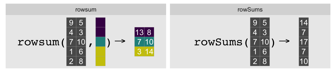
rowsum

I did mention this one in passing, but it bears re-examining: base::rowsum is a remarkable creature in the R ecosystem. As far as I know, it is the only base R function that computes group statistics on unequal group sizes in statically compiled code. Despite this it is arcane, especially when compared with its popular cousin base::rowSums.

rowsum and rowSums are near indistinguishable on name alone, but they do quite different things. rowsum collapses rows together by group, leaving column count unchanged, whereas rowSums collapses all columns leaving row count unchanged:

In the single column/vector case, rowsum(x, grp) computes the sum of x by the groups in grp. Typically this operation is done with tapply(x, grp, sum) (or vapply(split(x, grp), sum, 0)):

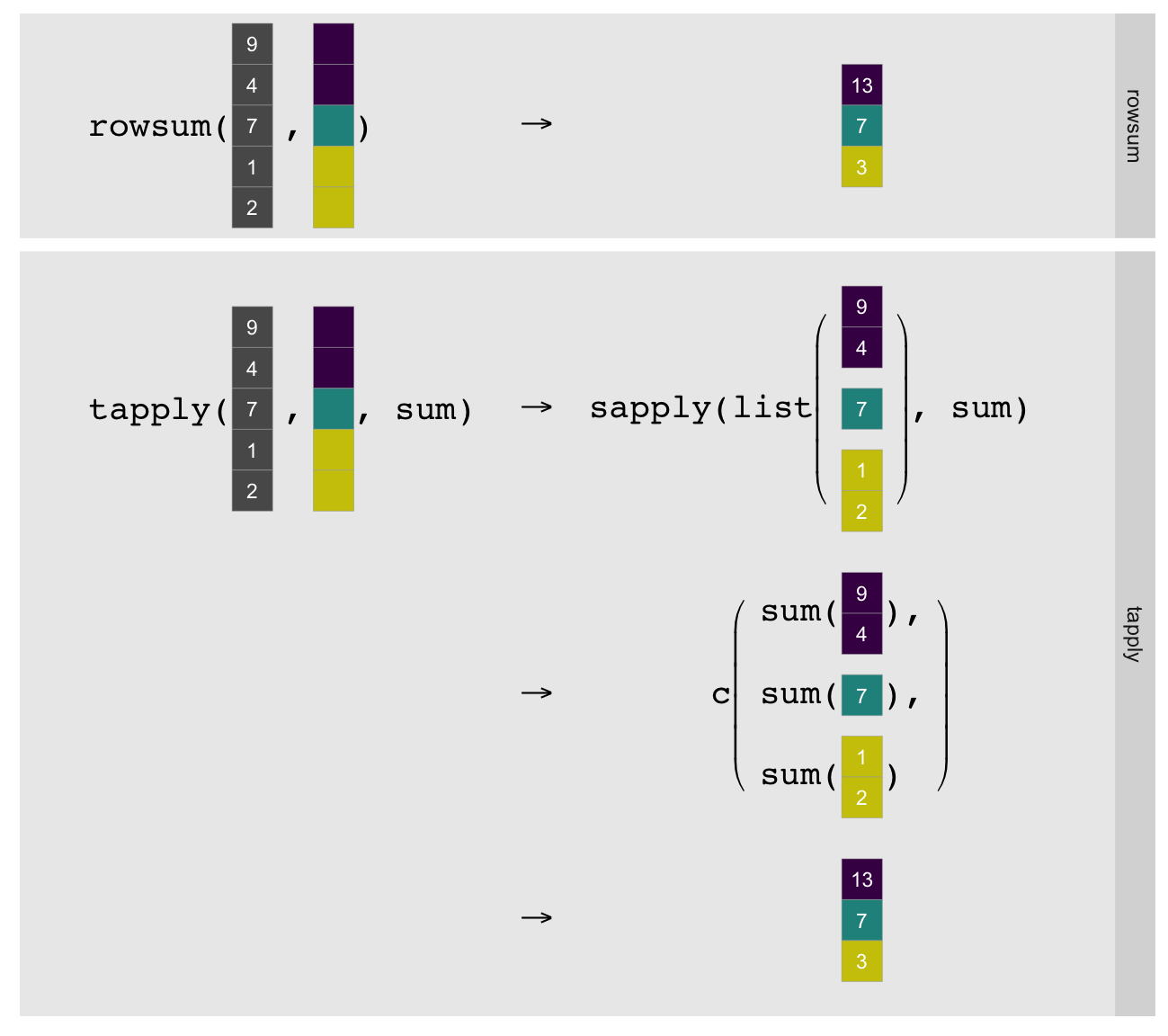
As illustrated above tapply must split the vector by group, explicitly call the R-level sum on each group, and simplify the result to a vector¹. rowsum can just compute the group sums directly in statically compiled code. This makes it substantially faster, although obviously limits it to computing sums.

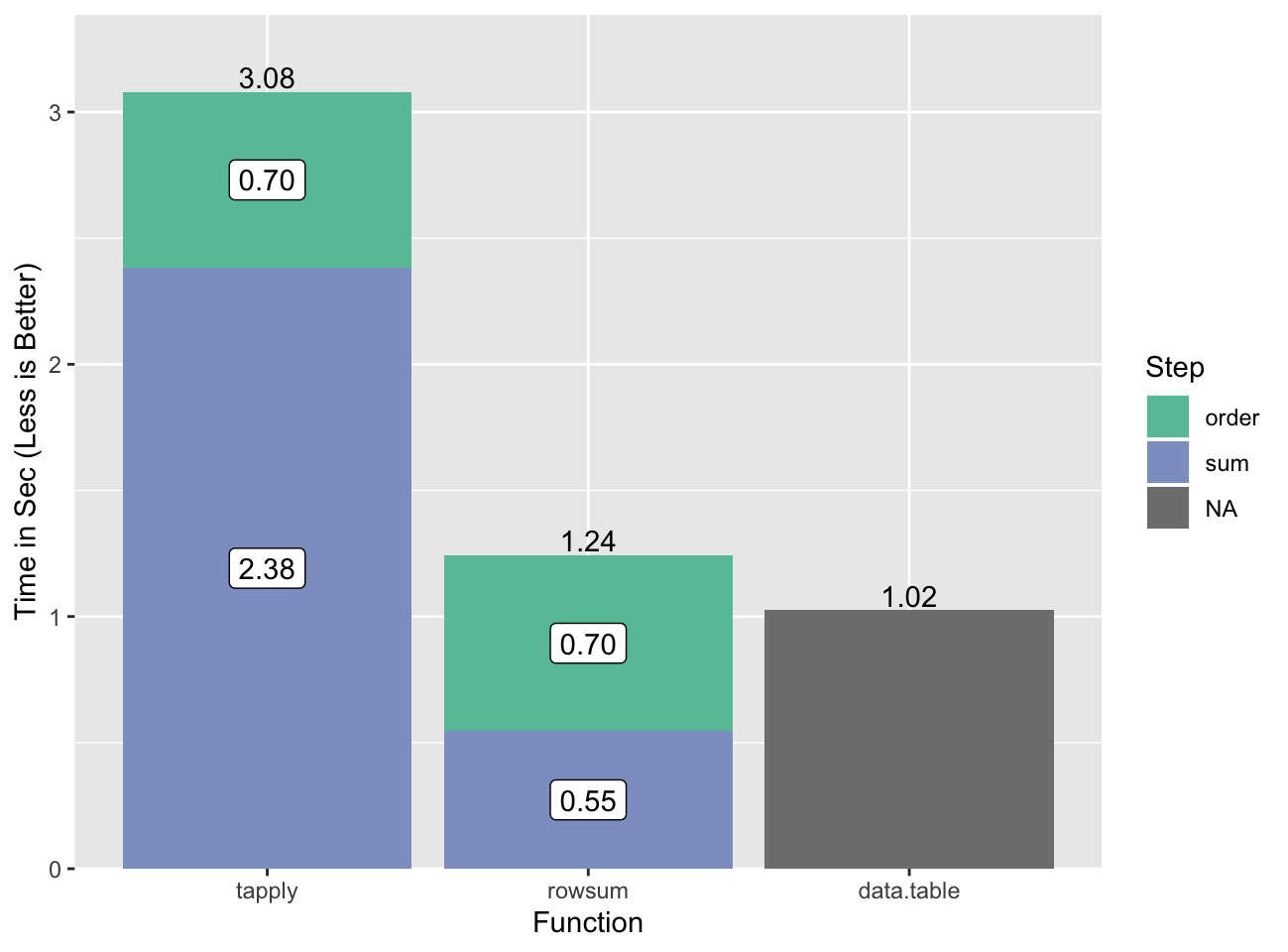
Let’s look at some examples and timings with our beaten-to-death 10MM row, ~1MM group data set, and our timing function sys.time. We’ll order the data first as that is fastest even when including the time to order:

sys.time({
  o <- order(grp)
  go <- grp[o]
  xo <- x[o]
})

   user  system elapsed
  0.690   0.003   0.696

tapply for reference:

sys.time(gsum.0 <- tapply(xo, go, sum))

   user  system elapsed
  2.273   0.105   2.383

And now rowsum:

sys.time(gsum.1 <- rowsum(xo, go))

   user  system elapsed
  0.507   0.038   0.546

all.equal(c(gsum.0), c(gsum.1), check.attributes=FALSE)

[1] TRUE

This is a ~4-5x speedup for the summing step, or a ~3x speedup if we include the time to order. data.table is faster for this task.

All data.table timings are single threaded (setDTthreads(1))².

The slow step for data.table is also the ordering, but we don’t have a good way to break that out.

colSums

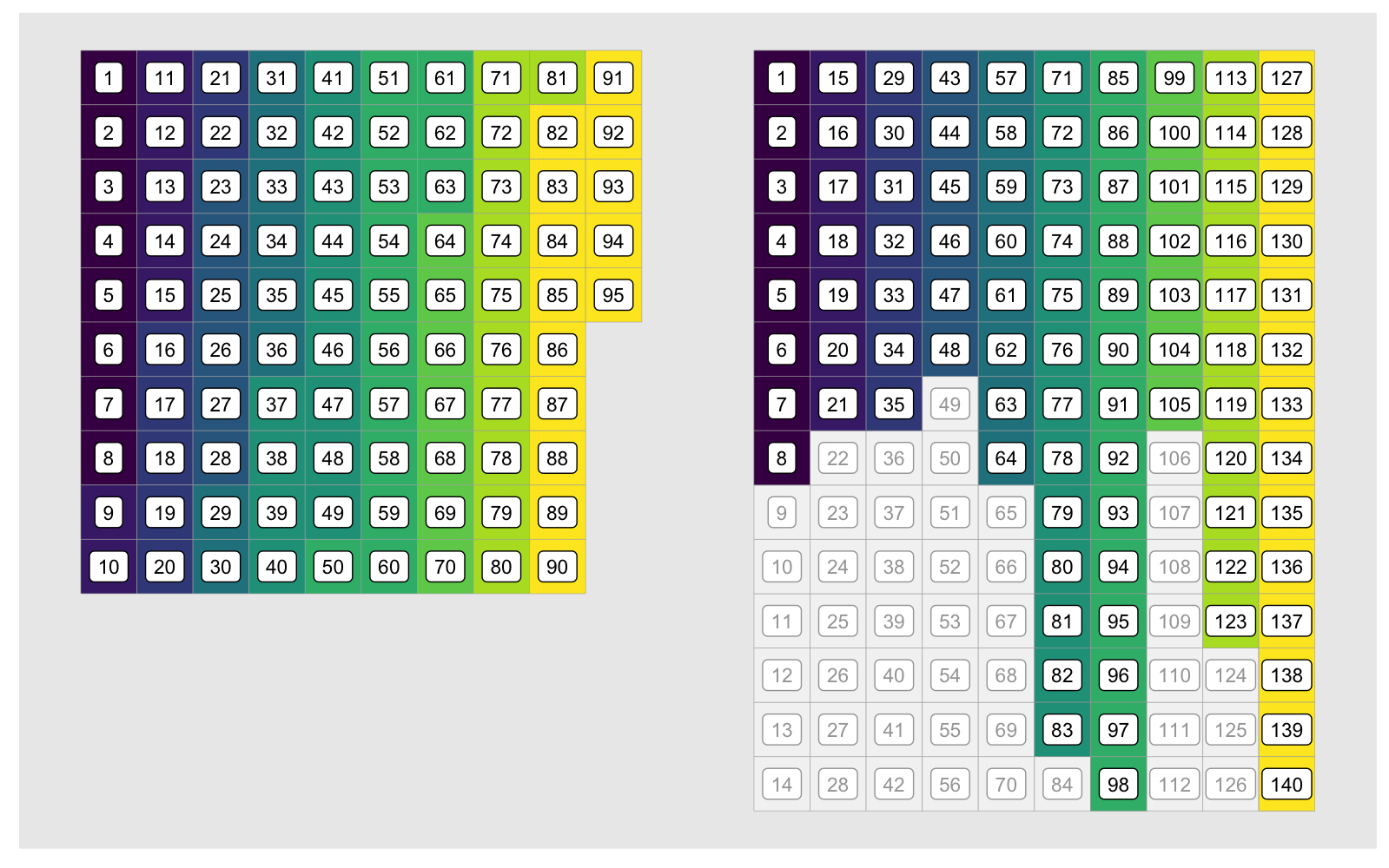
base::rowSums, the aforementioned better-known cousin of rowsum, also computes group statistics with statically compiled code. Well, it kind of does if you consider matrix rows to be groups. base::colSums does the same except for columns. Suppose we have three equal sized ordered groups:

(G <- rep(1:3, each=2))

[1] 1 1 2 2 3 3

And values that belong to them:

set.seed(1)
(a <- runif(6))

[1] 0.266 0.372 0.573 0.908 0.202 0.898

We can compute the group sums using colSums by wrapping our vector into a matrix with as many columns as there are groups. Since R internally stores matrices as vectors in column-major order, this is a natural operation (and also why we use colSums instead of rowSums):

(a.mx <- matrix(a, ncol=length(unique(G))))

      [,1]  [,2]  [,3]
[1,] 0.266 0.573 0.202
[2,] 0.372 0.908 0.898

colSums(a.mx)

[1] 0.638 1.481 1.100

This is equivalent to³:

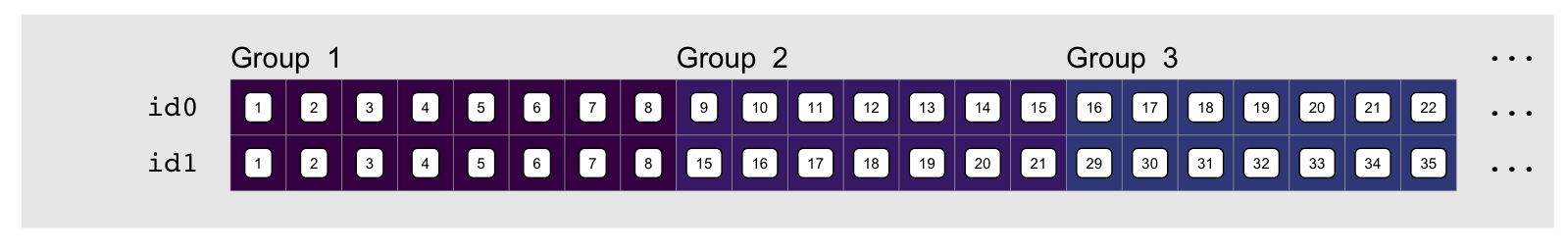
c(rowsum(a, G))

[1] 0.638 1.481 1.100

We run into problems as soon as we have uneven group lengths, but there is a workaround. The idea is to use clever indexing to embed the values associated with each group into columns of a matrix. We illustrate this process with a vector with 95 elements in ten groups. For display purposes we wrap the vector column-wise every ten elements, and designate the groups by a color. The values of the vector are represented by the tile heights:

This is an HTML Canvas flipbook that displays key frames of an animation in a more controllable manner than in a video player. If you are reading this text your browser does not support HTML Canvas.

    FPS:   #: / 15   ⤾:

You can also view the flipbook as a video if you prefer.

The embedding step warrants additional explanation. The trick is to generate a vector that maps the positions from our irregular vector into the regular matrix. There are several ways we can do this, but the one that we’ll use today takes advantage of the underlying vector nature of matrices. In particular, we will index into our matrices as if they were vectors, e.g.:

(b <- 1:4)

[1] 1 2 3 4

(b.mx <- matrix(b, nrow=2))

     [,1] [,2]
[1,]    1    3
[2,]    2    4

b[3]

[1] 3

b.mx[1, 2]   # matrix indexing

[1] 3

b.mx[3]      # vector indexing on matrix

[1] 3

Let’s look at our 95 data before and after embedding, showing the indices in vector format for both our ordered vector (left) and the target matrix (right):

The indices corresponding to each group diverge after the first group due to the unused elements of the embedding matrix, shown in grey above. What we’re looking for is a fast way to generate the indices in the colored cells in the matrix on the right. In other words, we want to generate the id1 (id.embed in the animation) vector below. For clarity we only show it for the first three groups:

We can emphasize the relationship between these by looking at the element by element difference in each index vector, e.g. using diff:

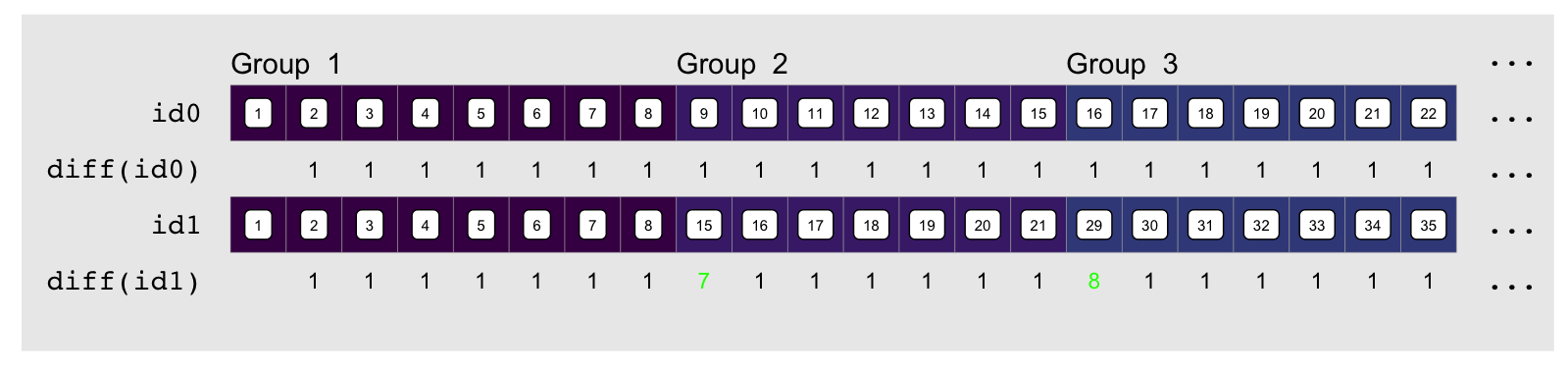
The indices always increment by one, except at group transitions for the embedding indices as shown in green above. There they increment by 1+pad. “pad” is how much empty space there is between the end of the group and the end of the column it is embedded in. The name of the game is to compute “pad”, which thankfully we can easily do by using the output of rle:

g.rle <- rle(sort(g))
g.rle

Run Length Encoding
  lengths: int [1:10] 8 7 7 6 8 13 14 7 11 14
  values : int [1:10] 1 2 3 4 5 6 7 8 9 10

rle gives us the length of runs of repeated values, which in our sorted group vector gives us the size of each group. Padding is then the difference between each group’s size and that of the largest group:

g.max <- max(g.rle[['lengths']])      # largest group
(pad <- g.max - g.rle[['lengths']])

 [1] 6 7 7 8 6 1 0 7 3 0

To compute the embedding vector we start by a vector of the differences which as a baseline are all 1:

id0 <- rep(1L, length(g))

We then add the padding at each group transition. Conveniently, the group transitions are just one element past the length of the previous element, so we can add the padding at the positions following the cumulative sum of the group lengths:

id0[cumsum(g.rle[['lengths']]) + 1L] <- pad + 1L
head(id0, 22)   # first three groups

 [1] 1 1 1 1 1 1 1 1 7 1 1 1 1 1 1 8 1 1 1 1 1 1

You’ll notice this is essentially the same thing as diff(id1) from earlier. We reproduce id1 by applying cumsum:

head(cumsum(id0), 22)

 [1]  1  2  3  4  5  6  7  8 15 16 17 18 19 20 21 29 30 31 32 33 34 35

A distinguishing feature of these manipulations other than possibly inducing death-by-boredom is that they are all in fast vectorized code. This gives us another reasonably fast group sum function. We split it up into a function that calculates the embedding indices and one that does the embedding and sum, for reasons that will become obvious later. Assuming sorted inputs⁴:

sys.time({
  emb <- og_embed_dat(go)   # compute embedding indices
  og_sum_col(xo, emb)       # use them to compute colSums
})

   user  system elapsed
  0.502   0.195   0.699

Most of the run time is actually the embedding index calculation:

sys.time(emb <- og_embed_dat(go))

   user  system elapsed
  0.369   0.141   0.510

One drawback is the obvious wasted memory taken up by the padding in the embedding matrix. This could become problematically large if a small number of groups are much larger than the rest. It may be possible to mitigate this by breaking up the data into by group size⁵.

Overall this is a little slower than rowsum for the simple group sum, but as we’ll see shortly there are benefits to this approach.

Pedal To The Metal

For the sake of an absolute benchmark I wrote a C version of rowsum, og_sum_C that takes advantage of group-ordered data to compute the group sums and counts⁶. Once the data is sorted, this takes virtually no time:

sys.time(og_sum_C(xo, go))

   user  system elapsed
  0.039   0.001   0.041

The only way to make this substantially faster is to make the sorting faster, or come up with an algorithm that can do the group sums without sorting and somehow do it faster than what we have here. Both of these are beyond my reach.

Let’s compare against all the different methods, including the original cumsum based group sum (cumsum-1), and the precision corrected two pass version (cumsum-2):

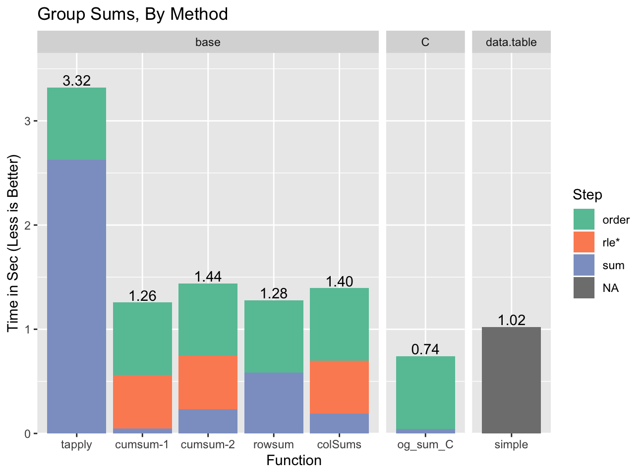
We’re actually able to beat data.table with our custom C code, although that is only possible because data.table contributed its fast radix sort to R, and data.table requires more complex code to be able to run a broader set of statistics.

The pattern to notice is that for several of the methods the time spent doing the actual summing is small⁷. For example, for colSums most of the time is ordering and computing the run length encoding / embedding indices (rle*). This is important because those parts can be re-used if the grouping is the same across several calculations. It doesn’t help for single variable group sums, but if we have more variables or more complex statistics it becomes a factor.

Let’s see how helpful re-using the group-based data is with the calculation of the slope of a bivariate regression:

∑(xi−ˉx)(yi−ˉy)∑(xi−ˉx)2

The calculation requires four group sums, two to compute ˉx and ˉy, and another two shown explicitly with the ∑ symbol. At the same time we only need to compute the ordering and the rle / embedding once because the grouping is the same across all calculations. You can see this clearly in the colSums based group slope calculation in the appendix.

When we compare all the previous implementations of the group slope calculation, against the new rowsum and colSums implementations the advantage of re-using the group information becomes apparent:

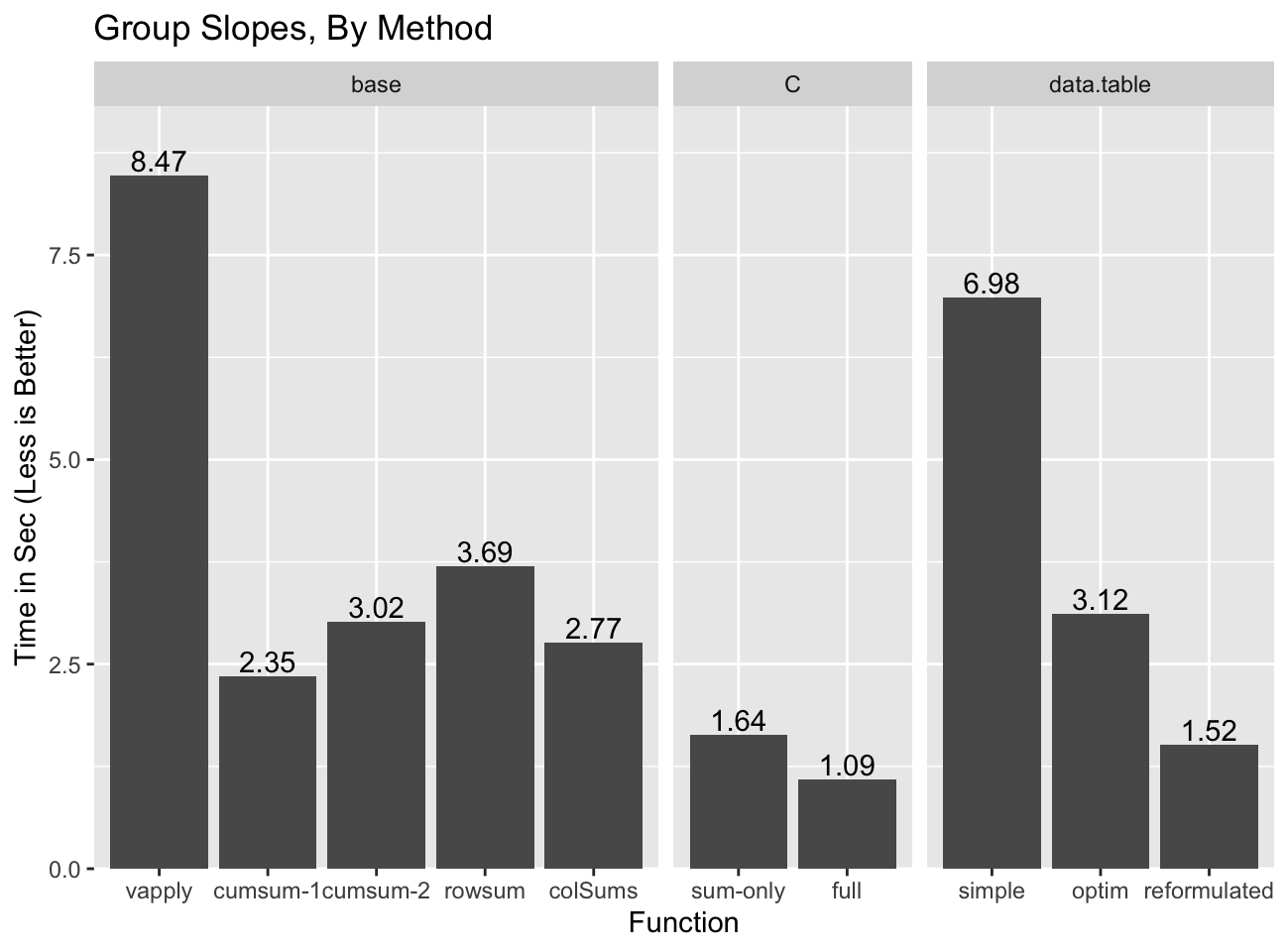
Even though rowsum was the fastest group sum implementation, it is the slowest of the base options outside of split/vapply because none of the computation components other than the re-ordering can be re-used. colSums does pretty well and has the advantage of not suffering from the precision issues of cumsum-1⁸, and additionally of naturally handling NA and non-finite values. cumsum-2⁹ might be the best bet of the “base” solutions as it is only slightly slower than colSums method, but should scale better if there are some groups that are much larger than most¹⁰.

data.table gets pretty close to the C implementation, but only in the reformulated form which comes with challenging precision issues.

That’s All Folks

Phew, finally done. I never imagined how out of hand some silly benchmarks against data.table would get. I learned way more than I bargained for, and come away from the whole thing with a renewed admiration for what R does: it can often provide near-statically-compiled performance in an interpreted language right out of the box¹¹. It’s not always easy to achieve this, but in many cases it is possible with a little thought and care.

This post is the last post of the Hydra Chronicles post series.

Appendix

sessionInfo()

R version 3.6.0 (2019-04-26)
Platform: x86_64-apple-darwin15.6.0 (64-bit)
Running under: macOS Mojave 10.14.6

Matrix products: default
BLAS:   /Library/Frameworks/R.framework/Versions/3.6/Resources/lib/libRblas.0.dylib
LAPACK: /Library/Frameworks/R.framework/Versions/3.6/Resources/lib/libRlapack.dylib

locale:
[1] en_US.UTF-8/en_US.UTF-8/en_US.UTF-8/C/en_US.UTF-8/en_US.UTF-8

attached base packages:
[1] stats     graphics  grDevices utils     datasets  methods   base     

other attached packages:
[1] data.table_1.12.2 gganimate_1.0.3   ggplot2_3.2.0     rayshader_0.11.5 

loaded via a namespace (and not attached):
 [1] rgl_0.100.19            Rcpp_1.0.1              prettyunits_1.0.2      
 [4] png_0.1-7               ps_1.3.0                assertthat_0.2.1       
 [7] rprojroot_1.3-2         digest_0.6.19           foreach_1.4.4          
[10] mime_0.7                R6_2.4.0                imager_0.41.2          
[13] tiff_0.1-5              plyr_1.8.4              backports_1.1.4        
[16] evaluate_0.14           blogdown_0.12           pillar_1.4.1           
[19] rlang_0.4.0             progress_1.2.2          lazyeval_0.2.2         
[22] miniUI_0.1.1.1          rstudioapi_0.10         callr_3.2.0            
[25] bmp_0.3                 rmarkdown_1.12          desc_1.2.0             
[28] devtools_2.0.2          webshot_0.5.1           servr_0.13             
[31] stringr_1.4.0           htmlwidgets_1.3         igraph_1.2.4.1         
[34] munsell_0.5.0           shiny_1.3.2             compiler_3.6.0         
[37] httpuv_1.5.1            xfun_0.8                pkgconfig_2.0.2        
[40] pkgbuild_1.0.3          htmltools_0.3.6         readbitmap_0.1.5       
[43] tidyselect_0.2.5        tibble_2.1.3            bookdown_0.10          
[46] codetools_0.2-16        crayon_1.3.4            dplyr_0.8.3            
[49] withr_2.1.2             later_0.8.0             grid_3.6.0             
[52] xtable_1.8-4            jsonlite_1.6            gtable_0.3.0           
[55] magrittr_1.5            scales_1.0.0            cli_1.1.0              
[58] stringi_1.4.3           farver_1.1.0            fs_1.3.1               
[61] promises_1.0.1          remotes_2.0.4           doParallel_1.0.14      
[64] testthat_2.1.1          iterators_1.0.10        tools_3.6.0            
[67] manipulateWidget_0.10.0 glue_1.3.1              tweenr_1.0.1           
[70] purrr_0.3.2             hms_0.4.2               crosstalk_1.0.0        
[73] jpeg_0.1-8              processx_3.3.1          pkgload_1.0.2          
[76] parallel_3.6.0          colorspace_1.4-1        sessioninfo_1.1.1      
[79] memoise_1.1.0           knitr_1.23              usethis_1.5.0          

RNGversion("3.5.2"); set.seed(42)
n     <- 1e7
n.grp <- 1e6
grp   <- sample(n.grp, n, replace=TRUE)
noise <- rep(c(.001, -.001), n/2)  # more on this later
x     <- runif(n) + noise
y     <- runif(n) + noise          # we'll use this later

# Run `system.time` `reps` times and return the timing closest to the median
# timing that is faster than the median.

sys.time <- function(exp, reps=11) {
  res <- matrix(0, reps, 5)
  time.call <- quote(system.time({NULL}))
  time.call[[2]][[2]] <- substitute(exp)
  gc()
  for(i in seq_len(reps)) {
    res[i,] <- eval(time.call, parent.frame())
  }
  structure(res, class='proc_time2')
}
print.proc_time2 <- function(x, ...) {
  print(
    structure(
      x[order(x[,3]),][floor(nrow(x)/2),],
      names=c("user.self", "sys.self", "elapsed", "user.child", "sys.child"),
      class='proc_time'
) ) }

og_embed_dat <- function(go) {
  ## compute run length encoding
  g.rle <- rle(go)
  g.lens <- g.rle[['lengths']]
  max.g <- max(g.lens)

  ## compute padding
  g.lens <- g.lens[-length(g.lens)]
  g.pad <- max.g - g.lens + 1L

  ## compute embedding indices
  id0 <- rep(1L, length(go))
  id0[(cumsum(g.lens) + 1L)] <- g.pad
  id1 <- cumsum(id0)

  list(idx=id1, rle=g.rle)
}

og_sum_col <- function(xo, embed_dat, na.rm=FALSE) {
  ## group sizes
  rle.len <- embed_dat[['rle']][['lengths']]

  ## allocate embedding matrix
  res <- matrix(0, ncol=length(rle.len), nrow=max(rle.len))

  ## copy data using embedding indices
  res[embed_dat[['idx']]] <- xo
  setNames(colSums(res, na.rm=na.rm), embed_dat[['rle']][['values']])
}

og_sum_C <- function(x, group) {
  stopifnot(
    typeof(x) == 'double', is.integer(group), length(x) == length(group)
  )
  tmp <- .og_sum_C(x, group)
  res <- setNames(tmp[[1]], tmp[[2]])
  attr(res, 'grp.size') <- tmp[[3]]
  res
}
.og_sum_C <- inline::cfunction(
  sig=c(x='numeric', g='integer'),
  body="
  R_xlen_t len, i, len_u = 1;
  SEXP res, res_x, res_g, res_n;
  int *gi = INTEGER(g);
  double *xi = REAL(x);
  len = XLENGTH(g);
  if(len != XLENGTH(x)) error(\"Unequal Length Vectors\");
  res = PROTECT(allocVector(VECSXP, 3));

  if(len > 1) {
    // count uniques
    for(i = 1; i < len; ++i) {
      if(gi[i - 1] != gi[i]) {
        ++len_u;
    } }
    // allocate and record uniques
    res_x = PROTECT(allocVector(REALSXP, len_u));
    res_g = PROTECT(allocVector(INTSXP, len_u));
    res_n = PROTECT(allocVector(INTSXP, len_u));

    double *res_xi = REAL(res_x);
    int *res_gi = INTEGER(res_g);
    int *res_ni = INTEGER(res_n);
    R_xlen_t j = 0;
    R_xlen_t prev_n = 0;

    res_xi[0] = 0;
    for(i = 1; i < len; ++i) {
      res_xi[j] += xi[i - 1];
      if(gi[i - 1] == gi[i]) {
        continue;
      } else if (gi[i - 1] < gi[i]){
        res_gi[j] = gi[i - 1];
        res_ni[j] = i - prev_n;  // this could overflow int; undefined?
        prev_n = i;
        ++j;
        res_xi[j] = 0;
      } else error(\"Decreasing group order found at index %d\", i + 1);
    }
    res_xi[j] += xi[i - 1];
    res_gi[j] = gi[i - 1];
    res_ni[j] = i - prev_n;

    SET_VECTOR_ELT(res, 0, res_x);
    SET_VECTOR_ELT(res, 1, res_g);
    SET_VECTOR_ELT(res, 2, res_n);
    UNPROTECT(3);
  } else {
    // Don't seem to need to duplicate x/g
    SET_VECTOR_ELT(res, 0, x);
    SET_VECTOR_ELT(res, 1, g);
    SET_VECTOR_ELT(res, 2, PROTECT(allocVector(REALSXP, 0)));
    UNPROTECT(1);
  }
  UNPROTECT(1);
  return res;
")

g_slope_col <- function(x, y, group) {
  ## order
  o <- order(group)
  go <- group[o]
  xo <- x[o]
  yo <- y[o]

  ## compute group means for x/y
  emb <- og_embed_dat(go)                    # << Embedding
  lens <- emb[['rle']][['lengths']]
  ux <- og_sum_col(xo, emb)/lens             # << Group Sum #1
  uy <- og_sum_col(yo, emb)/lens             # << Group Sum #2

  ## recycle means to input vector length and
  ##  compute (x - mean(x)) and (y - mean(y))
  gi <- rep(seq_along(ux), lens)
  x_ux <- xo - ux[gi]
  y_uy <- yo - uy[gi]

  ## Slope calculation
  gs.cs <-
    og_sum_col(x_ux * y_uy, emb) /           # << Group Sum #3
    og_sum_col(x_ux ^ 2, emb)                # << Group Sum #4
  setNames(gs.cs, emb[['rle']][['vaues']])
}
sys.time(g_slope_col(x, y, grp))

   user  system elapsed
  2.268   0.497   2.765

g_slope_C <- function(x, y, group) {
  stopifnot(
    typeof(x) == 'double', is.integer(group), length(x) == length(group),
    typeof(y) == 'double', length(x) == length(y)
  )
  o <- order(group)
  tmp <- .g_slope_C(x[o], y[o], group[o])
  res <- setNames(tmp[[1]], tmp[[2]])
  res
}
.g_slope_C <- inline::cfunction(
  sig=c(x='numeric', y='numeric',  g='integer'),
  body="
  R_xlen_t len, i, len_u = 1;
  SEXP res, res_x, res_g, res_y;
  int *gi = INTEGER(g);
  double *xi = REAL(x);
  double *yi = REAL(y);
  len = XLENGTH(g);
  if(len != XLENGTH(x)) error(\"Unequal Length Vectors\");
  res = PROTECT(allocVector(VECSXP, 2));

  if(len > 1) {
    // First pass compute unique groups
    for(i = 1; i < len; ++i) {
      if(gi[i - 1] != gi[i]) {
        ++len_u;
    } }
    // allocate and record uniques
    res_x = PROTECT(allocVector(REALSXP, len_u));
    res_y = PROTECT(allocVector(REALSXP, len_u));
    res_g = PROTECT(allocVector(INTSXP, len_u));

    double *res_xi = REAL(res_x);
    double *res_yi = REAL(res_y);
    int *res_gi = INTEGER(res_g);
    R_xlen_t j = 0;
    R_xlen_t prev_i = 0, n;

    // Second pass compute means

    double xac, yac;
    yac = xac = 0;
    for(i = 1; i < len; ++i) {
      xac += xi[i - 1];
      yac += yi[i - 1];
      if(gi[i - 1] == gi[i]) {
        continue;
      } else if (gi[i - 1] < gi[i]){
        n = i - prev_i;
        res_xi[j] = xac / n;
        res_yi[j] = yac / n;
        res_gi[j] = gi[i - 1];
        prev_i = i;
        yac = xac = 0;
        ++j;
      } else error(\"Decreasing group order found at index %d\", i + 1);
    }
    xac += xi[i - 1];
    yac += yi[i - 1];
    n = i - prev_i;
    res_xi[j] = xac / n;
    res_yi[j] = yac / n;
    res_gi[j] = gi[i - 1];

    // third pass compute slopes

    double xtmp, ytmp;
    yac = xac = xtmp = ytmp = 0;
    j = 0;

    for(i = 1; i < len; i++) {
      xtmp = xi[i - 1] -  res_xi[j];
      ytmp = yi[i - 1] -  res_yi[j];
      xac += xtmp * xtmp;
      yac += ytmp * xtmp;

      if(gi[i - 1] == gi[i]) {
        continue;
      } else {
        res_xi[j] = yac / xac;
        yac = xac = 0;
        ++j;
      }
    }
    xtmp = xi[i - 1] -  res_xi[j];
    ytmp = yi[i - 1] -  res_yi[j];
    xac += xtmp * xtmp;
    yac += ytmp * xtmp;
    res_xi[j] = yac / xac;

    SET_VECTOR_ELT(res, 0, res_x);
    SET_VECTOR_ELT(res, 1, res_g);
    UNPROTECT(3);
  } else {
    // Don't seem to need to duplicate x/g
    SET_VECTOR_ELT(res, 0, x);
    SET_VECTOR_ELT(res, 1, g);
    SET_VECTOR_ELT(res, 2, PROTECT(allocVector(REALSXP, 0)));
    UNPROTECT(1);
  }
  UNPROTECT(1);
  return res;
")