When Computing You Are Allowed to Cheat

Throughout the Hydra Chronicles we have explored why group statistics are problematic in R and how to optimize their calculation. R calls are slow, but normally this is not a problem because R will quickly hand off to native routines to do the heavily lifting. With group statistics there must be at least one R call per group. When there are many groups as in the 10MM row and ~1MM group data set we’ve been using, the R-level overhead adds up.

Both data.table and dplyr resolve the problem by providing native routines that can compute per-group statistics completely in native code for a limited number of statistics. This relies on the group expression being in the form statistic(variable) so that the packages may recognize the attempt to compute known group statistics and substitute the native code. There is a more complete discussion of this “Gforce” optimization in an earlier post. We can see it an action here:

library(data.table)
setDTthreads(1)            # for more stable timings

sys.time({                 # wrapper around sytem.time; see appendix
  DT <- data.table(x, grp)
  var.0 <- DT[, .(var=var(x)), keyby=grp]
})

   user  system elapsed
  1.890   0.024   1.923

sys.time is a wrapper around system.time defined in the appendix.

var.0

            grp    var
     1:       1 0.0793
     2:       2 0.0478
    ---               
999952:  999999 0.1711
999953: 1000000 0.0668

But what if we wanted the plain second central moment instead of the unbiased estimate produced by var:

\[E\left[\left(X - E[X]\right)^2\right]\]

Let’s start with the obvious method¹:

sys.time({
  DT <- data.table(x, grp)
  var.1 <- DT[, .(var=mean((x - mean(x)) ^ 2)), keyby=grp]
})

   user  system elapsed 
  4.663   0.049   4.728 

var.1

            grp    var
     1:       1 0.0721
     2:       2 0.0409
    ---               
999952:  999999 0.1466
999953: 1000000 0.0594

“Gforce” does not work with more complex expressions, so this ends up substantially slower. We can with some care break up the calculation into simple steps so that “Gforce” can be used, but this requires a group-join-group dance. There is an alternative: as Michael Chirico points out, sometimes we can reformulate a statistic into a different easier to compute form.

With the algebraic expansion:

\[(x - y)^2 = x^2 - 2 x y + y^2\]

And $c$ a constant (scalar), $X$ a variable (vector), $E[X]$ the expected value (mean) of $X$, and the following identities:

\[ \begin{align*} E[c] &= c\\ E\left[E[X]\right] &= E[X]\\ E[c X] &= c E[X]\\ E[X + Y] &= E[X] + E[Y] \end{align*} \]

We can reformulate the variance calculation:

\[ \begin{align*} Var(X) = &E\left[(X - E\left[X\right])^2\right]\\ = &E\left[X^2 - 2X E\left[X\right] + E\left[X\right]^2\right] \\ = &E\left[X^2\right] - 2 E\left[X\right]E\left[X\right] + E\left[X\right]^2 \\ = &E\left[X^2\right] - 2 E\left[X\right]^2 + E\left[X\right]^2 \\ = &E\left[X^2\right] - E\left[X\right]^2 \\ \end{align*} \]

The critical aspect of this reformulation is that there are no interactions between vectors and grouped values (statistics) so we can compute all the component statistics in a single pass. Let’s try it:

sys.time({
  DT <- data.table(x, grp)
  DT[, x2:=x^2]
  var.2 <- DT[,
    .(ux2=mean(x2), ux=mean(x)), keyby=grp  # grouping step
  ][,
    .(grp, var=ux2 - ux^2)                  # final calculation
  ]
})

   user  system elapsed 
  1.159   0.114   1.277 

all.equal(var.1, var.2)

[1] TRUE

Wow, that’s even faster than the “Gforce” optimized “var”. There is only one grouping step, and in that step all expressions are of the form statistic(variable) so they can be “Gforce” optimized.

These concepts apply equally to dplyr.

Beyond Variance

While it’s utterly fascinating (to some) that we can reformulate the variance computation, it’s of little value since both data.table and dplyr have compiled code that obviates the need for it. Fortunately this method is generally applicable to any expression that can be expanded and decomposed as we did with the variance. For example with a little elbow grease we can reformulate the third moment:

\[ \begin{align*} Skew(X) = &E\left[\left(X - E[X]\right)^3\right]\\ = & E\left[X^3 - 3 X^2 E\left[X\right] + 3 X E\left[X\right]^2 - E\left[X\right]^3\right]\\ = & E\left[X^3\right] - 3 E\left[X^2\right] E\left[X\right] + 3 E\left[X\right] E\left[X\right]^2 - E\left[X\right]^3\\ = & E\left[X^3\right] - 3 E\left[X^2\right] - 2E\left[X\right]^3 \end{align*} \]

And to confirm:

X <- runif(100)
all.equal(
  mean((X - mean(X))^3),
  mean(X^3) - 3 * mean(X^2) * mean(X) + 2 * mean(X) ^3
)

[1] TRUE

Similarly, and what set me off on this blogpost, it is possible to reformulate the slope of a single variable linear regression slope. What Michael Chirico saw that was not immediately obvious to me is that:

\[ \begin{align*} Slope(X,Y) = &\frac{Cov(X,Y)}{Var(X)}\\ = &\frac{ E\left[ \left(X - E\left[X\right]\right) \left(Y - E\left[Y\right]\right) \right] }{E\left[\left(X - E\left[X\right]\right)^2\right]}\\ = &\frac{ E\left[XY\right] - E\left[X\right]E\left[Y\right]}{ E\left[X^2\right] - E\left[X\right]^2} \end{align*} \]

In data.table-speak:

DT <- data.table(x, y, xy=x*y, x2=x^2, grp)
slope.dt.re <- DT[,
  .(ux=mean(x), uy=mean(y), uxy=mean(xy), ux2=mean(x2)),
  keyby=grp
][,
  .(grp, slope=(uxy - ux*uy)/(ux2 - ux^2))
]

   user  system elapsed
  1.377   0.126   1.507

As with all the reformulations we’ve seen the key feature of this one is there is no interaction between grouped statistics and ungrouped ones, allowing a single grouping step. With the reformulation data.table is able to beat the cumsum based base-R method we studied in an earlier post:

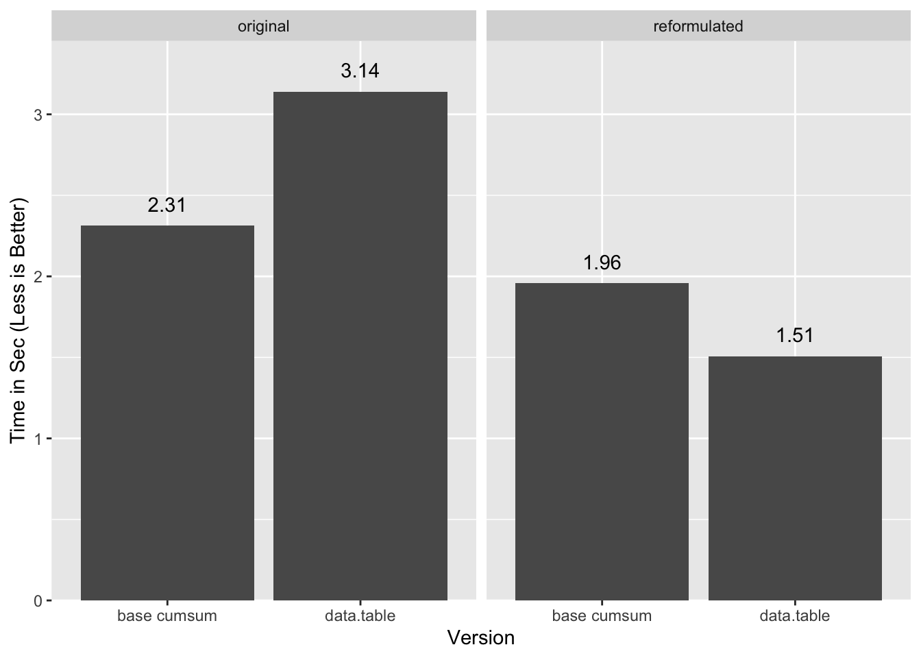
“Original” in this case is the single-pass cumsum method for base and the group-join-group method for data.table.

More generally we should be able to apply this expansion to any nested statistics involving sum or mean and possibly other functions, which will cover a broad range of interesting statistics. In the case of sum, keep in mind that:

\[ \sum_i^n c = n c \]

And similarly:

\[ \sum_i^n \left(c + X\right) = n c + \sum_i^n X \]

Slow Down Cowboy

Before we run off and reformulate all the things, it is worth noting that the wikipedia page I took the reformulation of the variance from also provides a scary warning:

This equation should not be used for computations using floating point arithmetic because it suffers from catastrophic cancellation if the two components of the equation are similar in magnitude.

Uh-oh. Let’s see:

quantile(((var.2 - var.3) / var.2), na.rm=TRUE)

       0%       25%       50%       75%      100%
-2.09e-07 -5.91e-16  0.00e+00  5.94e-16  2.91e-09

We did lose some precision, but certainly nothing catastrophic. So under what circumstances do we actually need to worry? Let’s cook up an example that actually causes a problem, as with these values at the edge of precision of double precision numbers.

X <- c(2^52 + 1, 2^52 - 1)
mean(X)

[1] 4.5e+15

mean((X - mean(X))^2)            # "normal" calc

[1] 1

mean(X^2) - mean(X)^2            # "reformulated" calc

[1] 0

If we carry out the algebraic expansion of the first element of $X^2$ we can see that problems crop up well before the subtraction:

\[ \begin{align*} (X_1)^2 = &(2^{52} + 2^0)^2\\ = &(2^{52})^2 + 2 \times 2^{52} \times 2^0 + (2^0)^2\\ = &2^{104} + 2^{53} + 2^0 \end{align*} \]

Double precision floating point numbers only have 53 bits of precision in the fraction, which means the difference between the highest power of two and the lowest one contained in a number cannot be greater than 52 without loss of precision. Yet, here we are trying to add $2^0$ to a number that contains $2^{104}$! This is completely out of the realm of what double precision numbers can handle:

identical(
  2^104 + 2^53,
  2^104 + 2^53 + 2^0
)

[1] TRUE

One might think, “oh, that’s just the last term, it doesn’t matter”, but it does:

\[ \require{cancel} \begin{align*} E[X^2] = &\frac{1}{N}\sum X^2\\ = &\frac{1}{2}\left(\left(2^{52} + 2^0\right)^2 + \left(2^{52} - 2^0\right)^2\right)\\ = &\frac{1}{2} \left(\left(\left(2^{104} \cancel{+ 2^{53}} + 2^0\right)\right) + \left((2^{104} \cancel{- 2^{53}} + 2^0)\right)\right)\\ = &2^{104} + 2^0 \end{align*} \]

The contributions from the middle terms cancel out, leaving only the last term as the difference between $E[X^2]$ and $E[X]^2$.

In essence squaring of $X$ values is causing meaningful precision to overflow out of the double precision values. By the time we get to the subtraction in $E[X^2] - E[X]^2$ the precision has already been lost. While it is true that $E[X^2]$ and $E[X]^2$ are close in the cases of precision loss, it is not the subtraction that is the problem.

Generally we need to worry when $\left|E[X]\right| \gg Var(X)$. The point at which catastrophic precision loss happens will be around $\left|E[X]\right| / Var(X) \approx 26$, as that is when squaring $X$ values will cause most or all the variance precision to overflow. We can illustrate with a sample with $n = 100$, $Var(X) = 1$, and varying ratios of $\left|E[X]\right| / Var(X)$, repeating the experiment 100 times for each ratio:

The flat lines that start forming around $2^{26}$ correspond to when overflow causes the reformulation to “round down” to zero. The more dramatic errors correspond to the last bit(s) rounding up instead of down². As the last bits are further and further in magnitude from the true value, the errors get dramatic.

If we know what the true $\left|E[X]\right| / Var(X)$ ratio is, we can estimate the likely loss of precision. Unfortunately we cannot get a correct measure of this value from the reformulated calculations. For example, if the true ratio is $2^{50}$, due to the possibility for gross overestimation the measured ratio might be as low as $2^2$:

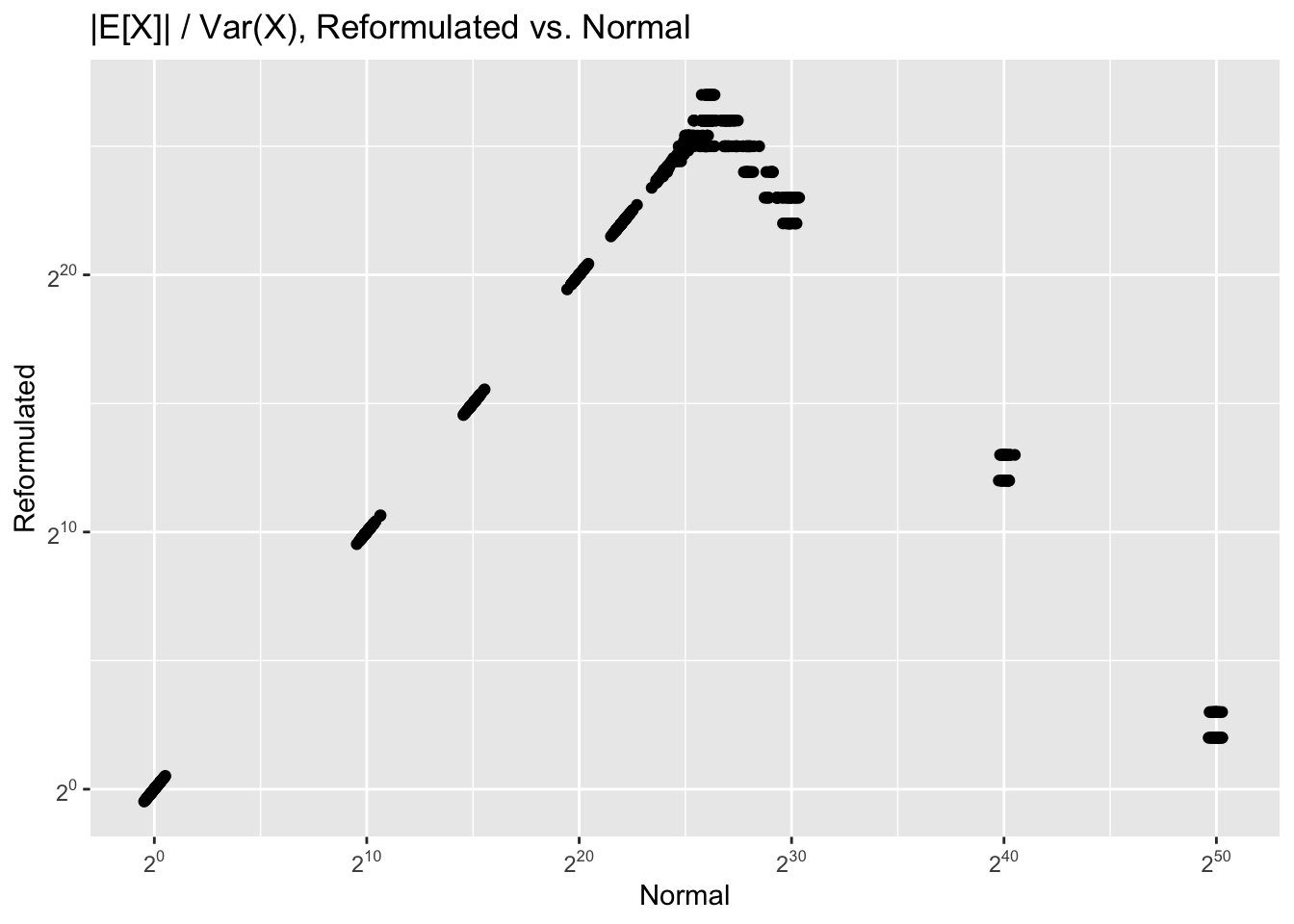
Infinite values (i.e. zero measured variance) are removed from the plot.

Another way to look at the precision loss is to examine the underlying binary representation of the floating point numbers. We do so here for each of the 100 samples of each of the attempted $\left|E[X]\right| / Var(X)$ ratios:

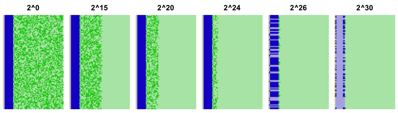
The fraction of the numbers is shown in green, and the exponent in blue. Dark squares are ones and dark ones zeroes. The precision loss shows up as trailing zeroes in those numbers (light green). This view makes it obvious that there is essentially no precision by the time we get to $\left|E[X]\right| / Var(X) \approx 26$, which is why the errors in the reformulation start getting so wild. We can estimate a lower bound on the precision by inspecting the bit pattern, but since there may be legitimate trailing zeroes this will likely be an under-estimate. See the appendix for a method that checks a number has at least n bits of precision.

Each reformulation will bring its own precision challenges. The skew calculation will exhibit the same overflow problems as the variance, except further exacerbated by the cube term. The slope reformulation introduces another wrinkle due to the division of the covariance by the variance. We can illustrate with variables $X$ and $Y$ each with true variance 1, and means $2^{26}$ and $2^4$ respectively. We sampled from these 100 values, 100 times, and plot the resulting bit patterns for the resulting finites slopes:

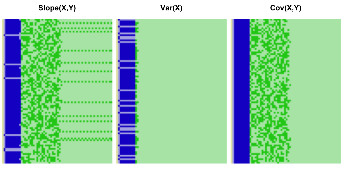
The precision of the overall calculation should be limited by that of the variance, but the interaction between the variance and covariance in all cases causes the bit pattern to overstate the available precision. In some cases, it even gives the illusion that all 53 bits are in use.

Unlike with our cumsum based group sum, I have not found a good way to estimate a bound on precision loss. The bit pattern method is likely our best bet, yet it feels… shaky. Not to mention that for large enough group counts it will produce false positives as some groups will randomly have statistics with many legitimate trailing zeroes.

A saving grace might be that, e.g. for the variance, data for which $\left|E[X]\right| \gg Var(X)$ should be reasonably rare. In cases where that might hold true, we will often have a rough order-of-magnitude estimate of $E[X]$ which we can subtract from the data prior to computation, though this is only useful if the mean is roughly the same across all groups³.

Conclusions

Reformulations is a powerful tool for dealing with group statistics, but the precision issues are worrying because they are difficult to measure, and may take new forms with each different reformulation.

Appendix

sessionInfo()

R version 3.6.0 (2019-04-26)
Platform: x86_64-apple-darwin15.6.0 (64-bit)
Running under: macOS Mojave 10.14.6

Matrix products: default
BLAS:   /Library/Frameworks/R.framework/Versions/3.6/Resources/lib/libRblas.0.dylib
LAPACK: /Library/Frameworks/R.framework/Versions/3.6/Resources/lib/libRlapack.dylib

locale:
[1] en_US.UTF-8/en_US.UTF-8/en_US.UTF-8/C/en_US.UTF-8/en_US.UTF-8

attached base packages:
[1] stats     graphics  grDevices utils     datasets  methods   base     

other attached packages:
[1] data.table_1.12.2 dplyr_0.8.3      

loaded via a namespace (and not attached):
 [1] Rcpp_1.0.1        magrittr_1.5      usethis_1.5.0     devtools_2.0.2   
 [5] tidyselect_0.2.5  pkgload_1.0.2     R6_2.4.0          rlang_0.4.0      
 [9] tools_3.6.0       pkgbuild_1.0.3    sessioninfo_1.1.1 cli_1.1.0        
[13] withr_2.1.2       remotes_2.0.4     assertthat_0.2.1  rprojroot_1.3-2  
[17] digest_0.6.19     tibble_2.1.3      crayon_1.3.4      processx_3.3.1   
[21] purrr_0.3.2       callr_3.2.0       fs_1.3.1          ps_1.3.0         
[25] testthat_2.1.1    memoise_1.1.0     glue_1.3.1        compiler_3.6.0   
[29] pillar_1.4.1      desc_1.2.0        backports_1.1.4   prettyunits_1.0.2
[33] pkgconfig_2.0.2  

sys.time({
  var.2a <- tibble(x, grp) %>%
    mutate(x2=x^2) %>%
    group_by(grp) %>%
    summarise(ux2=mean(x2), ux=mean(x)) %>%
    mutate(var=ux2 - ux^2) %>%
    select(grp, var)
})

   user  system elapsed 
 11.171   0.299  11.660 

all.equal(as.data.frame(var.2), as.data.frame(var.2a))

[1] TRUE

RNGversion("3.5.2"); set.seed(42)
n     <- 1e7
n.grp <- 1e6
grp   <- sample(n.grp, n, replace=TRUE)
noise <- rep(c(.001, -.001), n/2)  # more on this later
x     <- runif(n) + noise
y     <- runif(n) + noise          # we'll use this later

# Run `system.time` `reps` times and return the timing closest to the median
# timing that is faster than the median.

sys.time <- function(exp, reps=11) {
  res <- matrix(0, reps, 5)
  time.call <- quote(system.time({NULL}))
  time.call[[2]][[2]] <- substitute(exp)
  gc()
  for(i in seq_len(reps)) {
    res[i,] <- eval(time.call, parent.frame())
  }
  structure(res, class='proc_time2')
}
print.proc_time2 <- function(x, ...) {
  print(
    structure(
      x[order(x[,3]),][floor(nrow(x)/2),],
      names=c("user.self", "sys.self", "elapsed", "user.child", "sys.child"),
      class='proc_time'
) ) }

# requires double `x` of length > 0, and positive scalar `bits`
# assumes little endian byte order.  Not tested with NA or infinite values.

has_precision_bits <- function(x, bits) {
  n <- 53 - min(c(bits-1, 53))
  mask.full <- n %/% 8
  mask.extra <- n %% 8
  mask <- as.raw(c(
    rep(255, mask.full),
    if(mask.extra) 2^(mask.extra) - 1,
    rep(0, 8 - (mask.full + (mask.extra > 0)))
  ) )
  colSums(matrix(as.logical(writeBin(x, raw()) & mask), nrow=8)) > 0
}