Recap
mtcars in binary.
Last week we slugged it out with the reigning group-stats heavy weight
champ data.table. The challenge was to compute the slope of a bivariate
regression fit line over 10MM entries and ~1MM groups. The formula is:
\[\frac{\sum(x_i - \bar{x})(y_i - \bar{y})}{\sum(x_i - \bar{x})^{2}}\]
While this may seem like a silly task, we do it because computing group
statistics is both useful and a weakness in R. We implemented
group_slope based on John Mount’s cumsum idea, and for
a brief moment we thought we scored an improbable win over
data.table1. Unfortunately our results did not withstand
scrutiny.
Here is the data we used:
RNGversion("3.5.2"); set.seed(42)
n     <- 1e7
n.grp <- 1e6
grp   <- sample(n.grp, n, replace=TRUE)
noise <- rep(c(.001, -.001), n/2)  # more on this later
x     <- runif(n) + noise
y     <- runif(n) + noise          # we'll use this later
The slow and steady base R approach is to define the statistic as a function,
split the data, and apply the function with vapply or similar.
slope <- function(x, y) {
  x_ux <- x - mean.default(x)
  y_uy <- y - mean.default(y)
  sum(x_ux * y_uy) / sum(x_ux ^ 2)
}
id <- seq_along(grp)
id.split <- split(id, grp)
slope.ply <- vapply(id.split, function(id) slope(x[id], y[id]), 0)
Our wild child version is 4-6x faster, and should produce the same results. It doesn’t quite:
slope.gs <- group_slope(x, y, grp)  # our new method
all.equal(slope.gs, slope.ply)
[1] "Mean relative difference: 0.0001161377"With a generous tolerance we find equality:
all.equal(slope.gs, slope.ply, tolerance=2e-3)[1] TRUEDisclaimer: I have no special knowledge of floating point precision issues. Everything I know I learned from research and experimentation while writing this pots. If your billion dollar Mars lander burns up on entry because you relied on information in this post, you only have yourself to blame.
Oh the Horror!
As we’ve alluded to previously group_slope is running into precision issues,
but we’d like to figure out exactly what’s going wrong. Let’s find the group
with the worst relative error, which for convenience we’ll call B. Its index
in the group list is then B.gi:
B.gi <- which.max(abs(slope.gs / slope.ply))
slope.gs[B.gi]
616826
-3014.2slope.ply[B.gi] 616826
-2977.281That’s a ~1.2% error, which for computations is downright ghastly, and on an entirely different plane of existence than the comparatively quaint2:
1 - 0.7 == 0.3[1] FALSELet’s look at the values in our problem group 616826. It turns out there are
only two of them:
x[grp == 616826][1] 0.4229786 0.4229543y[grp == 616826][1] 0.7637899 0.8360645The x values are close to each other, but well within the resolution of the
double precision format (doubles henceforth), which are what R “numeric”
values are stored as. It gets a bit worse though because the next step is
$\sum(x - \bar{x})^2$:
(B.s <- sum((x[grp == 616826] - mean(x[grp == 616826]))^2))[1] 0.0000000002946472Still, nothing too crazy. In order to see why things go pear shaped we need to
look back at the algorithm we use in group_slope. Remember that we’re doing
all of this in vectorized code, so we don’t have the luxury of using things like
sum(x[grp == 616826]) where we specify groups explicitly to sum. Instead, we
use cumsum on group ordered data. Here is a visual recap of the key steps
(these are steps 4 and 5 of the previously described algorithm):
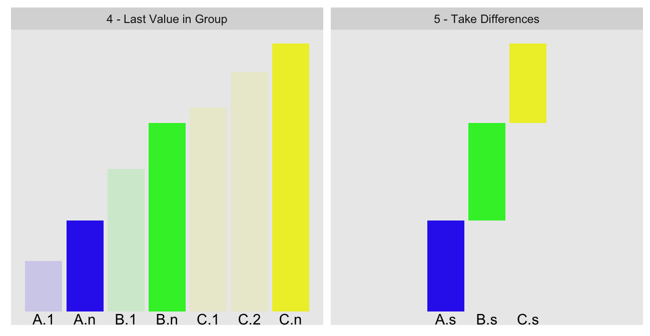
We use cumsum and some clever indexing to compute the values of A.n
(total cumulative sum of our group ordered statistic up to the last value before
our group B) and B.n (same quantity, but up to the last value in our group
B):
                    A.n                     B.n
462824.4016201458289288 462824.4016201461199671
To compute the group sum B.s, we take the difference of these two numbers.
Unfortunately, when values are so close to each other, doing so is the computing
equivalent of walking down the stairs into a dark basement with ominous
background music. To leave no doubt about the carnage that is about to unfold
(viewer discretion advised):
B.s.new <- B.n - A.n       # recompute B.s as per our algorithm
rbind(A.n, B.n, B.s.new)
[,1]
A.n 462824.4016201458289287984371185302734
B.n 462824.4016201461199671030044555664062
B.s.new 0.0000000002910383045673370361328
Doubles have approximately 15 digits of precision; we highlight those in green.
This would suggest B.s.new has no real precision left. At the same time, the
observed error of ~1.2% suggests there must be some precision. In
order to better understand what is happening we need to look at the true nature
of doubles.
Interlude — IEEE-754
Double precision floating points are typically encoded in base two in binary as per the IEEE-754 standard:
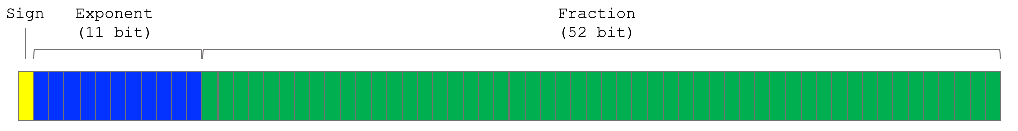
We’ll mostly use a mixed binary/decimal representation, where the fraction is shown in binary, and the exponent in decimal3:
+18     +10        0        -10       -20       -30 -34  <- Exponent (2^n)
 |       |         |         |         |         |   |
011100001111111010000110011011010000100100111110111111: A.n
011100001111111010000110011011010000100100111111000100: B.n
000000000000000000000000000000000000000000000000000101: B.s.new
For the sign bit 0 means positive and 1 means negative. Each power of two in
the fraction that lines up with a 1-bit is added to the value4. To
illustrate we can compute the integral value of A.n by adding
all the 1-bit powers of two with positive exponents from the fraction:
2^18 + 2^17 + 2^16 + 2^11 + 2^10 + 2^9 + 2^8 + 2^7 + 2^6 + 2^5 + 2^3[1] 462824This is not enough to differentiate between A.n and B.n. Even with all 52
bits5 we can barely tell the two numbers apart. As a result, when
we take the difference between those two numbers to produce B.s.new, most of
the fractions cancel out and leaving only three bits of precision6.
The actual encoding of B.s.new will have an additional 50 trailing zeroes, but
those add no real precision.
What about all those digits of seeming precision we see in the decimal
representation of B.s.new? Well check this out:
2^-32 + 2^-34[1] 2.910383045673370361328e-10B.s.new[1] 2.910383045673370361328e-10The entire precision of B.s is encapsulated in $2^{-32} + 2^{-34}$.
All those extra decimal digits are just an artifact of the conversion to
decimal, not evidence of precision.
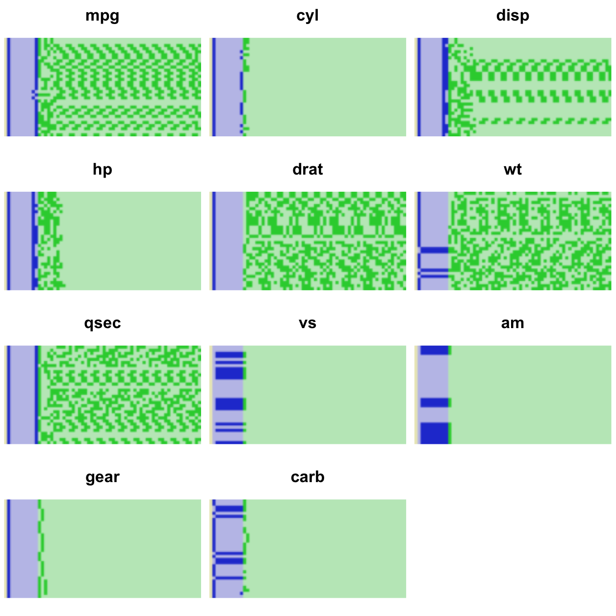
iris data set makes for a good
illustration as most measures are taken to one decimal place. Let’s look at it
in full binary format (plotting code in appendix):
iris underlying binary representation, big endian
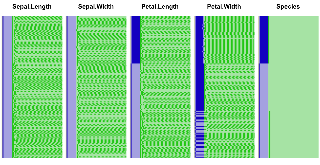
As in our previous illustration the sign bit (barely visible) is shown in yellow, the exponent in blue, and the fraction in green. Dark colors represent 1-bits, and light ones 0-bits. Let’s zoom into the first ten elements of the second column:

And the corresponding decimal values:
iris$Sepal.Width[1:10] [1] 3.5 3.0 3.2 3.1 3.6 3.9 3.4 3.4 2.9 3.1The first two elements are an integer and a decimal ending in .5. These can
be represented exactly in binary form, as is somewhat implicit in the trailing
zeroes in the first two rows7. The other numbers cannot be
represented exactly, as is implicit in the use of every available bit. We can
also see this by showing more digits in the decimals:
options(digits=18)
iris$Sepal.Width[1:10]
[1] 3.50000000000000000 3.00000000000000000 3.20000000000000018
[4] 3.10000000000000009 3.60000000000000009 3.89999999999999991
[7] 3.39999999999999991 3.39999999999999991 2.89999999999999991
[10] 3.10000000000000009Before we move on, it’s worth remembering that there is a difference between recorded precision and measured precision. There is zero chance that every iris measured had dimensions quantized in millimeters. The measurements themselves have no precision past the first decimal, so that the binary representation is only correct 15 decimal places or so is irrelevant for the purposes of this and most other data. The additional precision is mostly used as a buffer so that we need not worry about precision loss in typical computations.
How Bad Is It, Really?
Given the binary representation of our numbers, we should be able to estimate
what degree of error we could observe. The last significant bit in A.n and
B.n corresponds to $2^{-34}$, so at the limit each could be off by as much
as $\pm2^{-35}$. It follows that B.s, which is the difference of A.n and
B.n, could have up to twice the error:
\[2 \times \pm2^{-35} = \pm2^{-34}\]
With a baseline value of B.s of $2^{-32} + 2^{-34}$, the relative error
becomes8:
\[\pm\frac{2^{-34}}{2^{-32} + 2^{-34}} = \pm20\%\]
If the theoretical precision is only $\pm20\%$, how did we end up with only a
$~1.2\%$ error? Sheer luck, it turns out.
Precisely because cumsum is prone precision issues, R internally uses an
80 bit extended precision double for the accumulator. The 80 bit
values are rounded down to 64 bits prior to return to R. Of the additional 15
bits 10 are added to the fraction9.
Let’s look again at the A.n and B.n values, but this time comparing the
underlying 80 bit representations with the 64 bit one visible from R, first for A.n:
+18     +10        0        -10       -20       -30       -40
 |       |         |         |         |         |   *     |   *
01110000111111101000011001101101000010010011111011111100000000000:  64 bit
01110000111111101000011001101101000010010011111011111011100000101:  80 bit
00000000000000000000000000000000000000000000000000000000010111011: A.n Err
The extended precision bits are shown in light green. The additional bit beyond that is the guard bit used in rounding10.
And B.n:
+18     +10        0        -10       -20       -30       -40
 |       |         |         |         |         |   *     |   *
01110000111111101000011001101101000010010011111100010000000000000:  64 bit
01110000111111101000011001101101000010010011111100001111111000100:  80 bit
00000000000000000000000000000000000000000000000000000000000111100: B.n Err
The rounding errors A.n.err and B.n.err between the 80 and 64 bit
representations are small compared to the difference between the A.n and
B.n. Additionally, the rounding errors are in the same direction. As a
result the total error caused by the rounding from 80 bits to 64 bits, in
“binary” representation, should be $(0.00111100 - 1.01111011) \times 2^{-38}$,
or a hair under $2^{-38}$:
A.n.err.bits <- c(1,0,1,1,1,0,1,1)
B.n.err.bits <- c(0,0,1,1,1,1,0,0)
exps <- 2^-(38:45)
(err.est <- sum(B.n.err.bits * exps) - sum(A.n.err.bits * exps))
[1] -3.609557e-12Our estimate of the error matches almost exactly the actual error:
(err.obs <- B.s.new - B.s)[1] -3.608941e-12We can do a reasonable job of predicting the bounds of error, but what good is it to know that our result might be off by as much as 20%?
A New Hope
Before we give up it is worth pointing out that precision loss in some cases is
a feature. For example, Drew Schmidt’s float package implements single
precision numerics for R as an explicit trade-off of precision for memory and
speed. In deep learning, reduced precision is all the rage. In a sense,
we are trading off precision for speed in our cumsum group sums approach,
though not explicitly.
Still, it would be nice if we could make a version of this method that
doesn’t suffer from this precision infirmity. And it turns out we can! The
main source of precision loss is due to the accumulated sum eventually growing
much larger than any given individual group in size. This became particularly
bad for cumulative sum of $(x - \bar{x})^2$ due to the squaring
that exacerbates relative magnitude differences.
A solution to our problem is to use a two-pass calculation. The first-pass is as before, producing the imprecise group sums. In the second-pass we insert the negative of those group sums as additional values in each group:
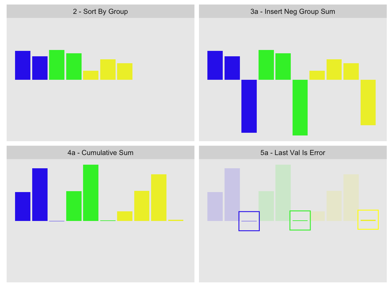
If the first-pass group sum was fully precise, the values inside the highlighting boxes in the last panel should be zero. The small values we see inside the boxes represent the errors of each group computation11. We can then take those errors and add them back to the first-pass group sums.
While the second-pass is still subject to precision issues, these are greatly reduced because the cumulative sum is reset to near zero after each group. This prevents the accumulator from becoming large relative to the values.
.group_sum_int2 below embodies the approach. One slight modification from the
visualization is that we subtract the first-pass group value from the last value
in the group instead of appending it to the group:
.group_sum_int2 <- function(x, last.in.group){
  x.grp <- .group_sum_int(x, last.in.group)     # imprecise pass
  x[last.in.group] <- x[last.in.group] - x.grp  # subtract from each group
  x.grp + .group_sum_int(x, last.in.group)      # compute errors and add
}
We can use it with group_slope2, a variation on group_slope
that can accept custom group sum functions:
sys.time(slope.gs2 <- group_slope2(x, y, grp, gsfun=.group_sum_int2)) user system elapsed
2.248 0.729 2.979 sys.time returns the median time of eleven runs of system.time, and is
defined in our previous post.
all.equal(slope.ply, slope.gs2)[1] TRUEquantile((slope.ply - slope.gs2)/slope.ply, na.rm=TRUE) 0% 25% 50% 75% 100%
-1.91e-12 0.00e+00 0.00e+00 0.00e+00 8.90e-12 This does not match the original calculations exactly, but there is essentially no error left. Compare to the single pass calculation:
quantile((slope.ply - slope.gs)/slope.ply, na.rm=TRUE) 0% 25% 50% 75% 100%
-1.24e-02 -1.92e-11 -2.16e-15 1.92e-11 8.33e-05 The new error is ten orders of magnitude smaller than the original.
Two-pass precision improvement methods have been around for long time. For
example R’s own mean uses a variation on this method.
If you are still wondering how we came up with the 80 bit representations of the
cumulative sums earlier, wonder no more. We use a method similar
to the above, where we compute the cumulative sum up to A.n, append the
negative of A.n and find the representation error for A.n. We than add that
error back by hand to the 64 bit representation12. Same thing for
B.n.
I Swear, It’s a Feature
We noted earlier that precision loss can be a feature. We can make it so in
this case by providing some controls for it. We saw earlier that it is possible
to estimate precision loss, so we can use this decide whether
we want to trigger the second precision correcting pass. .group_sum_int3 in
the appendix does exactly this by providing a
p.bits parameter. This parameter specifies the minimum number of bits of
precision in the resulting group sums. If as a result of the first pass we
determine the worst case loss could take us below p.bits, we run the second
precision improvement pass:
To illustrate we will time each of the group sum functions against the $(x - \bar{x})^2$ which we’ve stored in the x_ux2 variable:
microbenchmark::microbenchmark(times=10,
  .group_sum_int(x_ux2, gnc),            # original single pass
  .group_sum_int2(x_ux2, gnc),           # two pass, always
  .group_sum_int3(x_ux2, gnc, p.bits=2), # check, single pass
  .group_sum_int3(x_ux2, gnc, p.bits=3)  # check, two pass
)
Unit: milliseconds
expr min lq mean median uq max neval
.group_sum_int(x_ux2, gnc) 44.0 94.5 101 97 115 153 10
.group_sum_int2(x_ux2, gnc) 196.2 258.2 277 271 294 365 10
.group_sum_int3(x_ux2, gnc, p.bits = 2) 79.7 119.4 119 126 128 133 10
.group_sum_int3(x_ux2, gnc, p.bits = 3) 294.5 308.3 324 312 349 371 10In this example the worst case precision is 2 bits, so with p.bits=2 we run in
one pass, whereas with p.bits=3 two passes are required. There is some
overhead in checking precision, but it is small enough relative to the cost of
the second pass.
Let’s try our slope calculation, this time again demanding at least 16 bits of
precision. For our calculation 16 bits of precision implies the error will be
at most $\pm2^{-16} \approx \pm1.53 \times 10^{-5}$.
.group_sum_int_16 <- function(x, last.in.group)
  .group_sum_int3(x, last.in.group, p.bits=16)

sys.time(slope.gs3 <- group_slope2(x, y, grp, gsfun=.group_sum_int_16))
user system elapsed
2.052 0.652 2.706 all.equal(slope.ply[!is.na(slope.ply)], slope.gs3[!is.na(slope.ply)])[1] TRUEquantile((slope.ply - slope.gs3) / slope.ply, na.rm=TRUE) 0% 25% 50% 75% 100%
-2.91e-08 -2.51e-14 0.00e+00 2.51e-14 4.73e-09Indeed the errors are no larger than that13. The precision check occurs only at the group sum step, so if other steps steps accumulate errors it is possible for the final precision of a more complex computation to end up below the specified levels.
Verdict
Even with the precision correcting pass we remain faster than data.table under
the same formulation14:
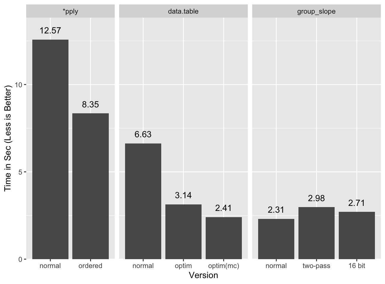
Applying the unconditional second pass is fast enough that the reduced precision version does not seem worth the effort. For different statistics it may be warranted.
Conclusions
I would classify this as a moral victory more than anything else. We can be as
fast as data.table, or at a minimum close enough, using base R only. When I
wrote the original group stats post I didn’t think we could get this
close. Mostly this is a curiosity, but for the rare cases where speedy group
stats are required and data.table is not available, we now know there is an
option.
One other important point in all this is that double precision floating point numbers are dangerous. They pack precision so far beyond typical measurements that it is easy to get lulled into a false sense of security about them. Yes, for the most part you won’t have problems, but there be dragons. For a more complete treatment of floating point precision issues see David Goldberg’s “What Every Computer Scientist Should Know About Floating-Point Arithmetic”.
Appendix
Updates
- 2019-07-25: Published bit pattern plotting code.
- 2019-06-23: Typos.
Acknowledgments
General
- Elio Campitelli for copy edits.
- Hadley Wickham and the
ggplot2authors forggplot2with which I made the plots in this post. - Olaf Mersmann etal. for creating microbenchmark, and Joshua Ulrich for maintaining it.
- Romain Francois for
seven31, which allowed I used when I first started exploring the binary representation of IEEE-754 double precision numbers. - Site acknowledgements.
Image Credits
- This floating point representation is a recreation of IEEE-754 Double Floating Point Format, by Codekaizen. It is recreated from scratch with a color scheme that better matches the rest of the post.
References
- David Goldberg, “What Every Computer Scientist Should Know About Floating-Point Arithmetic”, 1991.
- Richard M.Heiberger and Burt Holland, “Computational Precision and Floating Point Arithmetic”, Appendix G to “Statistical Analysis and Data Display”, Springer 2015, second edition.
Worst Case
If we had been unlucky maybe the true values of A.n and B.n would have been
as follows:
+18     +10        0        -10       -20       -30       -40
 |       |         |         |         |         |   *     |   *
01110000111111101000011001101101000010010011111011111100000000000: 64 bit
01110000111111101000011001101101000010010011111011111010000000001: 80 bit
00000000000000000000000000000000000000000000000000000001111111111: A.n Err
And:
+18     +10        0        -10       -20       -30       -40
 |       |         |         |         |         |   *     |   *
01110000111111101000011001101101000010010011111100010000000000000: 64 bit
01110000111111101000011001101101000010010011111100010010000000000: 80 bit
10000000000000000000000000000000000000000000000000000010000000000: B.n Err
These have the same 64 bit representations as the original values, but the error relative to the “true” 80 bit representations is quite different:
A.n.err.bits <- c(0,1,1,1,1,1,1,1,1,1,1)
B.n.err.bits <- -c(1,0,0,0,0,0,0,0,0,0,0)  # note this is negative
exps <- 2^-(35:45)

(err.est.max <- sum(B.n.err.bits * exps) - sum(A.n.err.bits * exps))
[1] -5.817924e-11err.est.max / B.s[1] -0.1974539err.obs / B.sIn this case we get roughly the maximum possible error, which is ~16 times larger than the observed one.
Functions and Computations
Adjustable Precision Group Sums
We take a worst-case view of precision loss, comparing the highest magnitude we reach in our cumulative sums to the smallest magnitude group. This function does not account for NA or Inf values, although it should be possible to adapt it as per our previous post.
.group_sum_int3 <- function(x, last.in.group, p.bits=53, info=FALSE) {
  xgc <- cumsum(x)[last.in.group]
  gmax <- floor(log2(max(abs(range(xgc)))))
  gs <- diff(c(0, xgc))
  gsabs <- abs(gs)
  gmin <- floor(log2(min(gsabs[gsabs > 0])))
  precision <- 53 + (gmin - gmax)
  if(precision < p.bits) {
    x[last.in.group] <- x[last.in.group] - gs
    gs <- gs + .group_sum_int(x, last.in.group)
  }
  if(info) # info about precision and second pass
    structure(gs, precision=precision, precision.mitigation=precision < p.bits)
  else gs
}
group_slope2
Variation on group_slope that accepts alternate group sum functions.
group_slope2 <- function(x, y, grp, gsfun=.group_sum_int) {
  ## order inputs by group
  o <- order(grp)
  go <- grp[o]
  xo <- x[o]
  yo <- y[o]

  ## group sizes and group indices
  grle <- rle(go)
  gn <- grle[['lengths']]
  gnc <- cumsum(gn)              # Last index in each group
  gi <- rep(seq_along(gn), gn)   # Group recycle indices

  ## compute mean(x) and mean(y), and recycle them
  ## to each element of `x` and `y`:
  sx <- gsfun(xo, gnc)
  ux <- (sx/gn)[gi]
  sy <- gsfun(yo, gnc)
  uy <- (sy/gn)[gi]

  ## (x - mean(x)) and (y - mean(y))
  x_ux <- xo - ux
  y_uy <- yo - uy

  ## Slopes!
  x_ux.y_uy <- gsfun(x_ux * y_uy, gnc)
  x_ux2 <- gsfun(x_ux ^ 2, gnc)
  setNames(x_ux.y_uy / x_ux2, grle[['values']])
}
x_ux2
x_ux2 contains the group-ordered values of $(x - \bar{x})^2$. To compute it
we start by ordering the inputs and computing indices:
o <- order(grp)
go <- grp[o]
xo <- x[o]
grle <- rle(grp)
gn <- grle[['lengths']]
gnc <- cumsum(gn)
gi <- rep(seq_along(gn), gn)
We then compute $\bar{x}$ for each group, and use that for the final step:
ux <- .group_sum_int(xo, gnc) / gn
x_ux2 <- (xo - ux[gi])^2
Binary Representation Plots
This is definitely “I-did-the-bare-minimum-to-get-it-to-work-code”.
# This does not actually get the binary representation.  It infers it by
# calculation harcoding the NA and +zero cases, and leaving many others
# uncovered.  It would be much better to use @coolbutuseless's writeBin method,
# but since this more or less works...

val_to_bit <- function(x, start, end) {
  sig <- integer(start - end + 1L)
  exp <- floor(log2(x))
  exps <- start:end
  for(i in seq_along(exps)) if(sig[i] <- x >= 2^exps[i]) x <- x - 2^exps[i]
  sig
}
.bin_rep_int <- function(x) {
  x <- as.numeric(x)
  if(is.na(x)) {
    # we're just taking the 731 NA_real_ value, irrespecitve of what type of NA
    # we're dealing with
    as.integer(c(0, rep(1, 11), rep(0, 41), c(1,1,1,1,0,1,0,0,0,1,0)))
  } else if(x == 0) {
    integer(64)
  } else {
    positive <- x > 0
    x <- abs(x)
    exp <- floor(log2(x))
    significand <- val_to_bit(x, exp, exp - 52L)
    exponent <- val_to_bit(exp + 1023L, 10L, 0L)
    c(as.integer(!positive), exponent, significand[-1L])
  }
}
bin_rep <- function(x) {
  if(!all(is.finite(x)))
    stop("scalar finite non-na inputs only")
  structure(vapply(x, .bin_rep_int, integer(64)), class='bin_rep')
}
print.bin_rep <- function(x, ...) {
  apply(x, 2,
    function(y) {
      sign <- if(!y[1]) '+' else '-'
      writeLines(
        sprintf(
          "%s1.%s * 2^%d", sign,
          paste0(c(y[-(1:12)]), collapse=""),
          sum(2^(10:0) * y[2:12]) - 1023L
  ) ) } )
  invisible(NULL)
}
plot.bin_rep <- function(x, ...) {
  res <- array(0, c(dim(x), 3))

  fg0 <- .9
  bg0 <- .7
  fg1 <- .8
  bg1 <- .1

  # sign

  ind.sign.1 <- which(x & row(x) == 1, arr.ind=TRUE)
  ind.sign.0 <- which(!x & row(x) == 1, arr.ind=TRUE)

  res[cbind(ind.sign.1,3)] <- bg1
  res[rbind(cbind(ind.sign.1,1), cbind(ind.sign.1,2))] <- fg1
  res[cbind(ind.sign.0,3)] <- bg0
  res[rbind(cbind(ind.sign.0,1), cbind(ind.sign.0,2))] <- fg0

  ind.exp.1 <- which(x & row(x) %in% 2:11, arr.ind=TRUE)
  ind.exp.0 <- which(!x & row(x) %in% 2:11, arr.ind=TRUE)

  res[rbind(cbind(ind.exp.1,1), cbind(ind.exp.1,2))] <- bg1
  res[cbind(ind.exp.1,3)] <- fg1
  res[rbind(cbind(ind.exp.0,1), cbind(ind.exp.0,2))] <- bg0
  res[cbind(ind.exp.0,3)] <- fg0

  ind.frac.1 <- which(x & row(x) %in% 12:64, arr.ind=TRUE)
  ind.frac.0 <- which(!x & row(x) %in% 12:64, arr.ind=TRUE)

  res[rbind(cbind(ind.frac.1,1), cbind(ind.frac.1,3))] <- bg1
  res[cbind(ind.frac.1,2)] <- fg1
  res[rbind(cbind(ind.frac.0,1), cbind(ind.frac.0,3))] <- bg0
  res[cbind(ind.frac.0,2)] <- fg0

  # res[rep(rowSums(res, dims=2) == 0, 3)] <- 1
  # for(i in 10:1) res[i + 1,,] <- pmax(res[i + 1,,], i/20)
  # for(i in 1:52) res[i + 12,,] <- pmax(res[i + 12,,], i/104)

  plot(as.raster(unclass(aperm(res, c(2,1,3)))))
}
The win was for a literal implementation of the slope formula, under a reformulated version as shown by Michael Chirico
data.tableis faster.↩One quirk of IEEE-754 floating point numbers is that some decimals such as 0.3 and 0.7 cannot be represented exactly in the encoding. Some calculations such as this one expose that quirk.↩
We show the entire fraction, including the implicit leading bit, and we show the de-biased exponent explicitly. See the IEEE-754 wikipedia page for details.↩
Only the most significant bit’s exponent is recorded. We highlight that by coloring it differently. Note that for
B.s.new, the most significant exponent is actually -32, which is not shown here to try to keep the representation simple.↩If you counted closely you would see we show 53 bits in the fraction, not 52. This is because in reality “doubles” only store the last 52 bits of the fraction. The first unstored bit is always assumed to be 1, so 52 bits are encoded explicitly, and the additional 53rd implicitly. For clarity we show that first bit explicitly. There is an exception to the first bit assumption: when the exponent is all zeroes the first implicit bit will be assumed to be zero as well. This corresponds to “subnormal” numbers.↩
Internally the
B.swill be stored with all 53 bits of precision, but the trailing 50 bits will be all zeroes and carry no real precision.↩Integers of magnitude less than
$2^{53}$can be represented exactly, as well as any decimal that can be expressed as a negative power of two (e.g.$2^{-1} = 0.5$,$2^{-2} = 0.25$, etc.) or combination thereof for which the most significant bit is within 53 bits of the least significant one. Similarly a subset of integers larger than$2^{53}$can be represented exactly with the same constraint.↩The relative error value will fluctuate depending on the value we are measuring it to. Our reference value is in binary
1.01(exp:$2^{-32}$), but it could also have been1.11or0.01, so for 3 bit values the relative error can be as low as ~14% or as high as 100%.↩Unlike with normal double precision numbers, there is no implicit leading 1 bit in 80 bit extended precision, so even though there are 16 additional bits, there are only 15 effective additional bits.↩
It is unclear to me exactly when guard (and round and sticky) bits are available or not. Presumably they are part of the registers, so as long as numbers reside in them they are accessible. My experiments suggest this, but I was not able to find clear evidence this is actually the case.↩
We exaggerated the errors for expository purposes.↩
since R doesn’t support 80 bit doubles at the user level, we had to do the binary addition by hand…↩
We need to exclude NAs because in the comparisons because there are several groups where under full precision, we end up with the calculation
0/0 == NA, but under 16 bit precision we have0/(0 + 2^-16) == 0. That is, with some small error what would be an undefined slope becomes a zero slope.↩It is possible to reformulate the statistic to a form that allows
data.tableto be fastest, although that form has precision issues of its own.↩