Group Statistics in R

A known limitation of R is the substantial overhead to evaluate R expressions. Most workhorse functions hand off quickly to lean pre-compiled routines so this is usually not a problem, but we must be careful with R-level loops such as for, or *pply family¹. So long as the number of iterations is small relative to the data size, there is no problem. For example, looping through the columns of a 1,000,000 row by 10 column data frame is fine, but looping through the rows probably won’t be.

A common use case where this limitation is difficult to avoid is the computation of group statistics on data sets with many groups². This requires a minimum of one R function call for each group, and the additional overhead of splitting the input into groups in R objects.

For example, in:

x   <- c(1, 2, 3, 4, 6, 8, 16)
grp <- c('A', 'B', 'A', 'C', 'A', 'B', 'C')
tapply(x, grp, var)

    A     B     C 
 6.33 18.00 72.00 

tapply breaks up x according to the groups in grp and applies the var function to each of the resulting pieces of x. Conceptually you can visualize it as follows, with individual colored squares representing vector values and their colors the groups:

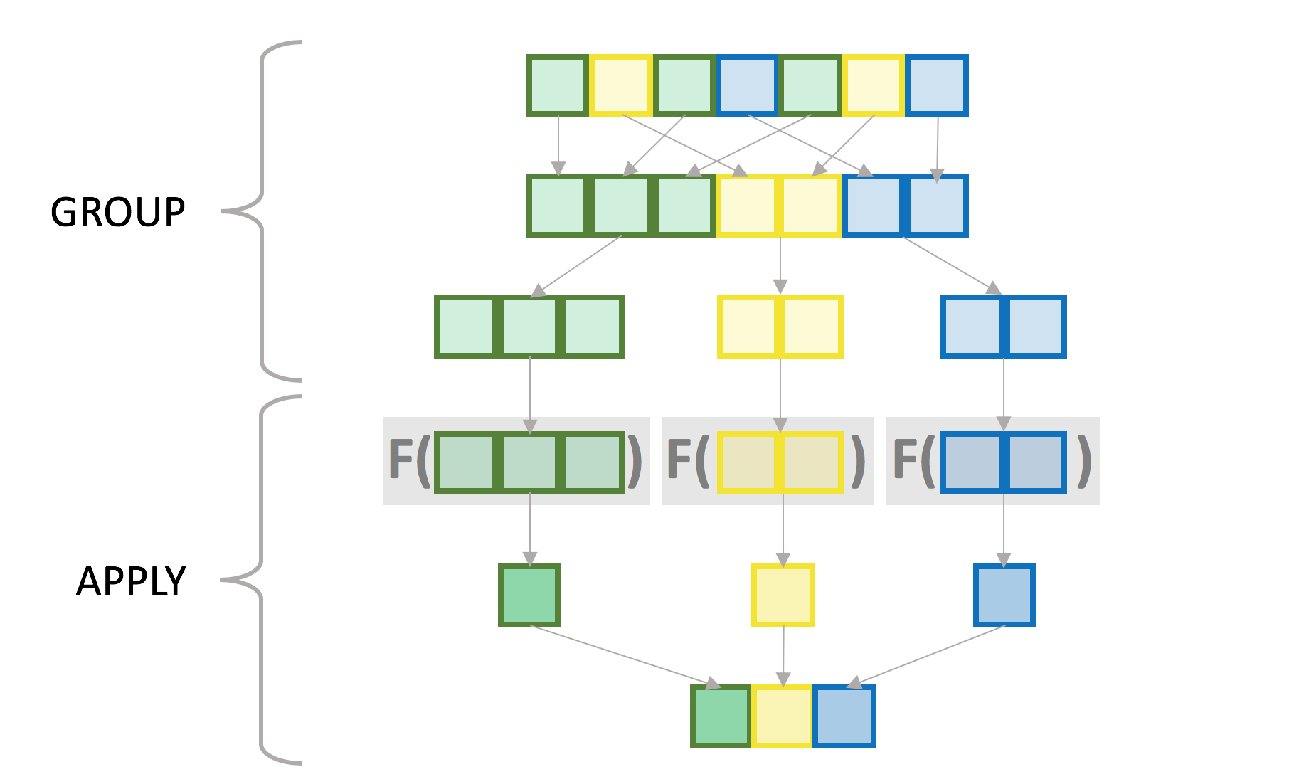
While this is not exactly what tapply is doing internally, particularly in the grouping step, the semantics are roughly the same. There is no requirement that the applied function should return a single value per group, although for the purposes of this post we are focusing on that type of function. The result of all this is a vector with as many elements as there are groups and with the groups as the names³.

Let’s try it again with something closer to “real data” size, in this case 10 million values and ~1 million groups⁴:

RNGversion("3.5.2"); set.seed(42)
n     <- 1e7
n.grp <- 1e6
grp   <- sample(n.grp, n, replace=TRUE)
x     <- runif(n)

system.time(x.grp <- tapply(x, grp, var))

   user  system elapsed
 48.933   0.787  50.474

Compare with:

system.time(var(x))

   user  system elapsed
  0.061   0.001   0.062

Note: Throughout this post I only show one run from system.time, but I have run the timings several times to confirm they are stable, and I show a representative run⁵.

Even though both commands are running a similar number of computations in compiled code⁶, the version that calls the R-level function once is several orders of magnitude faster than the one that calls it for each group.

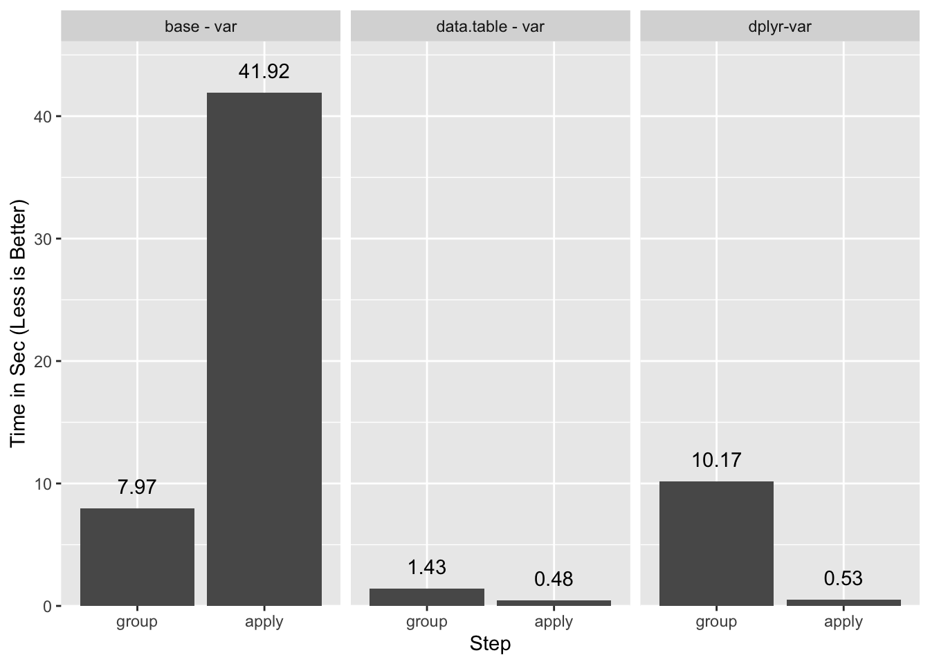
As alluded to earlier R call overhead is not the only difference between the two examples. tapply must also split the input vector into groups. To evaluate the relative cost of each task, we can separate the tapply call into its grouping (split) and apply components⁷. split breaks up the input vector into a list with one element for each group:

system.time(x.split <- split(x, grp))

   user  system elapsed
  7.124   0.617   7.966

str(x.split[1:3])   # show first 3 groups:

List of 3
 $ 1: num [1:11] 0.216 0.537 0.849 0.847 0.347 ...
 $ 2: num [1:7] 0.0724 0.1365 0.5364 0.0517 0.1887 ...
 $ 3: num [1:7] 0.842 0.323 0.325 0.49 0.342 ...

vapply then collapses each group into one number with the var statistic:

system.time(x.grp.2 <- vapply(x.split, var, 0))

   user  system elapsed
 40.001   0.629  41.921

str(x.grp.2)

 Named num [1:999953] 0.079 0.0481 0.0715 0.0657 0.0435 ...
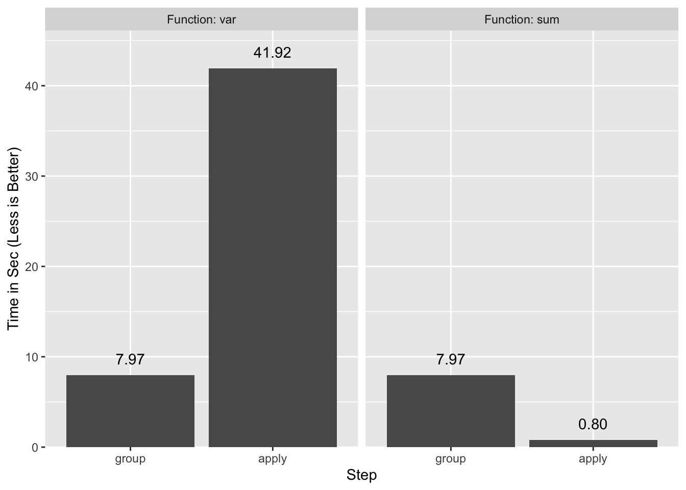
 - attr(*, "names")= chr [1:999953] "1" "2" "3" "4" ...

all.equal(c(x.grp), x.grp.2)

[1] TRUE

While the var computation accounts for the bulk of the elapsed time, the splitting can become significant with functions that are faster than var⁸. For example, with sum which is one of the lowest overhead statistics in R, the grouping becomes the limiting element:

system.time(vapply(x.split, sum, 0))

   user  system elapsed
  0.605   0.011   0.620

A side-by-side comparison of the two timings makes this obvious. The “group” timing is the same for both functions.

tapply is not the only function that computes group statistics in R, but it is one of the simpler and faster ones.

data.table to the Rescue

Thankfully the data.table package implements several optimizations to assist with this problem.

library(data.table)  # 1.12.0
setDTthreads(1)      # turn off data.table parallelization

Note: I turned off parallelization for data.table as it did not make a significance difference in this particular example, and it muddied the benchmarks⁹.

DT <- data.table(grp, x)
DT

             grp     x
       1: 914807 0.116
       2: 937076 0.734
      ---
 9999999: 714619 0.547
10000000: 361639 0.442

In order to compute a group statistic with data.table we use:

DT[, var(x), keyby=grp]

            grp     V1
     1:       1 0.0790
     2:       2 0.0481
    ---
999952:  999999 0.1707
999953: 1000000 0.0667

We use keyby instead of the traditional by because it instructs data.table to group and to order the return table by the groups, which matches what tapply does¹⁰. Timings are a different story:

system.time(x.grp.dt <- DT[, var(x), keyby=grp][['V1']])

   user  system elapsed
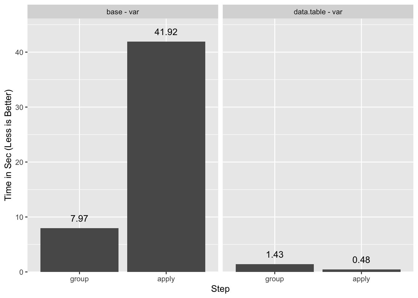
  1.821   0.062   1.909

all.equal(c(x.grp), x.grp.dt, check.attributes=FALSE)

[1] TRUE

We’ve reproduced the same results at ~25x the speed.

It is not possible to separate out the statistic computation cleanly from the grouping in data.table¹¹, but we can get a rough idea by setting a key on grp. This orders the table by the group, which is most of the overhead of grouping.

setkey(DT, grp)   # grouping takes advantage of this key
DT                # notice the table is now ordered by group

              grp     x
       1:       1 0.216
       2:       1 0.537
      ---
 9999999: 1000000 0.180
10000000: 1000000 0.919

What remains is mostly the statistic computation:

system.time(DT[, var(x), keyby=grp])

   user  system elapsed
  0.458   0.017   0.477

That step is close to two orders of magnitude faster than with vapply.

A summary of the timings:

What is this Sorcery?

How is it that data.table runs the R var function so much faster than vapply? vapply adds some overhead, but not much as shown when run with the essentially NULL-op unary +¹²:

system.time(vapply(1:1e6, `+`, 0L))

   user  system elapsed
  0.358   0.006   0.365

It turns out we are being lied to: data.table does not call the R var function ~1 million times. Instead it intercepts the call var(x) and substitutes it with a compiled code routine. This routine computes all the groups without intervening R-level evaluations. The data.table authors call this “GForce” optimization¹³.

The substitution is only possible if there is a pre-existing compiled code equivalent for the R-level function. data.table ships with such equivalents for the “base” R¹⁴ functions min, max, mean¹⁵, median, prod, sum, sd, var, head, tail¹⁶, and [¹⁷ as well as for the data.table functions first and last.

Additionally, the substitution only happens with the simplest of calls. Adding a mere unary + call causes it to fail:

system.time(DT[, +var(x), keyby=grp])

   user  system elapsed
 42.564   0.628  45.394

If you need a different function or a non-trivial expression you’ll have be content with falling back to standard evaluation. You can check whether data.table uses it by setting the verbose option¹⁸:

options(datatable.verbose=TRUE)
DT[, var(x), keyby=grp]

Detected that j uses these columns: x
Finding groups using uniqlist on key ... 0.113s elapsed (0.045s cpu)
Finding group sizes from the positions (can be avoided to save RAM) ... 0.020s elapsed (0.012s cpu)
lapply optimization is on, j unchanged as 'var(x)'
GForce optimized j to 'gvar(x)'
Making each group and running j (GForce TRUE) ...

And to confirm that adding the unary + disables “GForce”:

DT[, +var(x), keyby=grp]

Detected that j uses these columns: x
Finding groups using uniqlist on key ... 0.034s elapsed (0.029s cpu)
Finding group sizes from the positions (can be avoided to save RAM) ... 0.009s elapsed (0.009s cpu)
lapply optimization is on, j unchanged as '+var(x)'
GForce is on, left j unchanged
Old mean optimization is on, left j unchanged.
Making each group and running j (GForce FALSE)

Blood From a Turnip

Imagine we wish to compute the slope of a bi-variate least squares regression. The formula is:

\[\frac{\sum(x_i - \bar{x})(y_i - \bar{y})}{\sum(x_i - \bar{x})^{2}}\]

The R equivalent is:

slope <- function(x, y) {
  x_ux <- x - mean(x)
  uy <- mean(y)
  sum(x_ux * (y - uy)) / sum(x_ux ^ 2)
}

In order to use this function with the base split/*pply paradigm we need a little additional manipulation:

y <- runif(n)

system.time({
  id <- seq_along(grp)
  id.split <- split(id, grp)
  res.slope.base <- vapply(id.split, function(id) slope(x[id], y[id]), 0)
})

   user  system elapsed
 17.745   0.318  18.453

Instead of splitting a single variable, we split an index that we then use to subset each variable.

data.table makes this type of computation easy:

DT <- data.table(grp, x, y)
system.time(res.slope.dt1 <- DT[, slope(x, y), keyby=grp])

   user  system elapsed
 11.501   0.136  11.679

The timings improve over base, but not by the margins we saw previously. This is because data.table cannot use the sum and mean “GForce” counterparts when they are inside another function, or even when they are part of complex expressions.

So, what are we to do? Are we stuck writing custom compiled code?

Fortunately for us there is one last resort: with a little work we can break up the computation into pieces and take advantage of “GForce”. The idea is to compute intermediate values with mean and sum in simple calls that can use “GForce”, and carry out the rest of the calculations separately.

In this case, the rest of the calculations use the operators *, -, /, and ^.

These arithmetic operators have the property that their results are the same whether computed with or without groups. It follows that the lack of “GForce” counterparts for the operators is a non-issue.

We start by computing $\bar{x}$ and $\bar{y}$:

DT <- data.table(grp, x, y)
setkey(DT, grp)   # more on this in a moment
DTsum <- DT[, .(ux=mean(x), uy=mean(y)), keyby=grp]

Then we compute the $(x - \bar{x})$ and $(y - \bar{y})$ values by joining (a.k.a merging) our original table DT to the summary table DTsum with the $\bar{x}$ and $\bar{y}$ values. In data.table this can be done by subsetting for rows with another data.table¹⁹:

DT[DTsum, `:=`(x_ux=x - ux, y_uy=y - uy)]
DT

              grp     x     y    x_ux   y_uy
       1:       1 0.216 0.950 -0.3353 0.5058
       2:       1 0.537 0.914 -0.0146 0.4697
      ---
 9999999: 1000000 0.180 0.589 -0.3681 0.0109
10000000: 1000000 0.919 0.914  0.3711 0.3359

The `:=`(…) call adds columns to DT with the results of the computations, recycling the $\bar{x}$ and $\bar{y}$ from DTsum. In effect this is equivalent to a join-and-update. We could have achieved the same with the simpler:

DT <- data.table(grp, x, y)
DT[, `:=`(ux=mean(x), uy=mean(y)), keyby=grp]

While this works, it is much slower because it cannot use “GForce” as data.table does not implement it within :=. So instead we are stuck with the group to DTsum and the join to update DT.

If you look back you can see that we used setkey right before computing DTsum²⁰. We did this for two reasons:

1. setkey tells data.table what column to join on when we subset with another data.table as above, and it makes the join fast.
2. Keys can also be used to make grouping faster, so by setting the key early we used it both for the group and the join.

The rest is relatively straightforward:

DT[, `:=`(x_ux.y_uy=x_ux * y_uy, x_ux2=x_ux^2)]
DTsum <- DT[, .(x_ux.y_uy=sum(x_ux.y_uy), x_ux2=sum(x_ux2)), keyby=grp]
res.slope.dt2 <- DTsum[, .(grp, V1=x_ux.y_uy / x_ux2)]

And we get the same result as with the base solution:

all.equal(res.slope.base, res.slope.dt2[[2]], check.attributes=FALSE)

[1] TRUE

Let’s time the whole thing:

DT <- data.table(grp, x, y)
system.time({
  setkey(DT, grp)
  DTsum <- DT[, .(ux=mean(x), uy=mean(y)), keyby=grp]
  DT[DTsum, `:=`(x_ux=x - ux, y_uy=y - uy)]
  DT[, `:=`(x_ux.y_uy=x_ux * y_uy, x_ux2=x_ux^2)]
  DTsum <- DT[, .(x_ux.y_uy=sum(x_ux.y_uy), x_ux2=sum(x_ux2)), keyby=grp]
  res.slope.dt2 <- DTsum[, .(grp, V1=x_ux.y_uy / x_ux2)]
})

   user  system elapsed
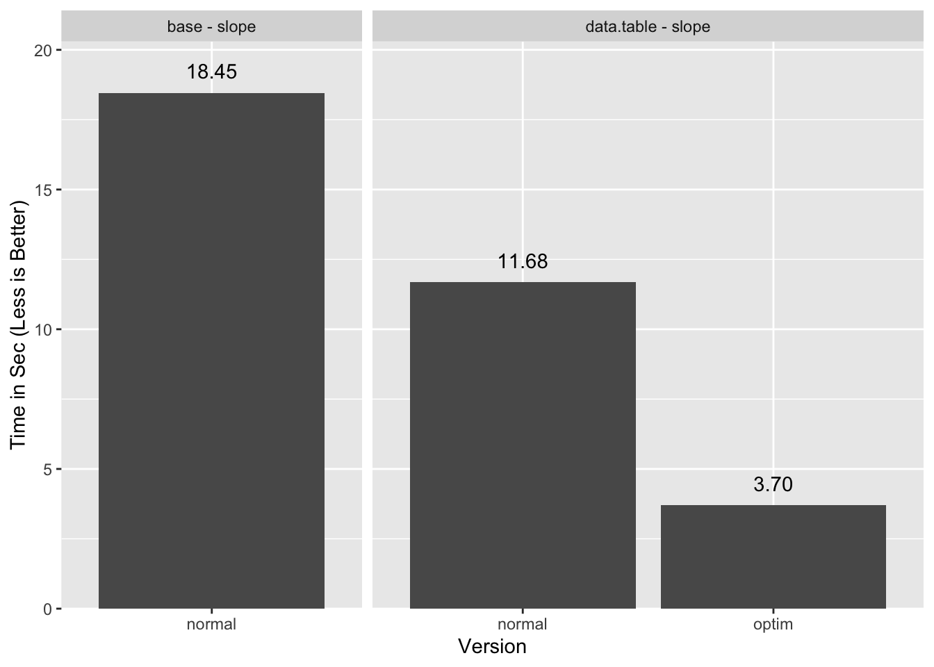
  3.278   0.403   3.697

A ~3x improvement over the unoptimized data.table solution, and a ~5x improvement over the base solution.

By carefully separating the computations into steps that can use “GForce” and steps that don’t need it to be fast, we are able to get “GForce”-like performance in an application for which that may seem impossible at first blush.

Should data.table add “GForce” support for := I estimate the timings could get down to 2.5 seconds or less²¹ with the cleaner but currently “GForce”-less alternate solution. Hopefully the authors will see it fit to implement this feature.

What About dplyr?

Like data.table, dplyr implements a “GForce” style evaluation. dplyr calls this “Hybrid Evaluation”²². For slow functions like var²³ this leads to substantial performance improvements over the base solution:

library(dplyr)
TB <- tibble(grp, x)
system.time(TB %>% group_by(grp) %>% summarize(var(x)))

   user  system elapsed
  9.823   0.609  10.639

Performance-wise the “Hybrid Evaluation” component is comparable to data.table’s “Gforce” and is responsible for the improvements over base’s performance:

TB.g <- TB %>% group_by(grp)
system.time(TB.g %>% summarize(var(x)))

   user  system elapsed
  0.521   0.003   0.527

On the whole dplyr underperforms data.table despite the competitive special evaluation because its grouping step is slower.

Since the dplyr “Hybrid Evaluation” is effective, we should be able to apply the same strategy as with data.table to optimize the computation of slope. Unfortunately it is an uphill battle as shown by the times of the baseline run:

TB <- tibble(grp, x, y)
system.time(res.dplyr1 <- TB %>% group_by(grp) %>% summarise(slope(x, y)))

   user  system elapsed
  32.65    1.39   34.51

With no attempted optimizations dplyr is ~3x slower than the equivalent data.table call and close to ~2x slower than the base version.

Due to the performance impact of group_by the best solution I found is somewhat convoluted. We’ll go through it in steps. First we compute the groups (TB.g) and $\bar{x}$ and $\bar{y}$. We save TB.g as we will re-use it later:

TB.g <- TB %>% group_by(grp)
TB.u <- TB.g %>% summarize(ux=mean(x), uy=mean(y))

Next is the join and computation of ungrouped stats:

TB.s <- TB %>%
  inner_join(TB.u, by='grp') %>%
  mutate(x_ux=x-ux, y_uy=y-uy, x_ux.y_uy=x_ux*y_uy, x_ux2=x_ux^2) %>%
  select(x_ux.y_uy, x_ux2)

# A tibble: 10,000,000 x 2
  x_ux.y_uy  x_ux2
      <dbl>  <dbl>
1   -0.0488 0.0157
2    0.0401 0.0212
# … with 1e+07 more rows

So far this is similar to what we did with data.table except we saved the intermediate statistics into their own table TB.s. We use that in the next step:

res.dplyr2 <- bind_cols(TB.g, TB.s) %>%
  summarise(x_ux.y_uy=sum(x_ux.y_uy), x_ux2=sum(x_ux2)) %>%
  ungroup %>%
  mutate(slope=x_ux.y_uy / x_ux2) %>%
  select(grp, slope)
res.dplyr2

# A tibble: 999,953 x 2
    grp  slope
  <int>  <dbl>
1     1 -0.706
2     2  0.134
# … with 1e+06 more rows

all.equal(res.slope.base, res.dplyr2[[2]], check.attributes=FALSE)

[1] TRUE

Rather than calling group_by on TB.s at the cost of ~10 seconds, we bind it to TB.g to re-use that tibble’s groups. This only works if the order of rows in TB.g and TB.s is the same. As far as I can tell dplyr does not support a group-ungroup-regroup²⁴ mechanism that would allow us to avoid the explicit re-grouping without having to resort to bind_cols.

Let’s time a slightly reworked but equivalent single-pipeline version:

system.time({
  TB.g <- TB %>% group_by(grp)
  res.dplyr2a <- TB.g %>%
    summarise(ux=mean(x), uy=mean(y)) %>%
    inner_join(TB, ., by='grp') %>%
    mutate(x_ux=x-ux, y_uy=y-uy, x_ux.y_uy=x_ux*y_uy, x_ux2=x_ux^2) %>%
    select(x_ux.y_uy, x_ux2) %>%
    bind_cols(TB.g, .) %>%
    summarise(x_ux.y_uy=sum(x_ux.y_uy), x_ux2=sum(x_ux2)) %>%
    ungroup %>%
    mutate(slope=x_ux.y_uy / x_ux2) %>%
    select(grp, slope)
})

   user  system elapsed
 16.256   0.974  17.591

This is slightly faster than the base solution.

I also tried a direct translation of the data.table optimization, but the repeated group_by makes it too slow. I also tried to avoid the join by using mutate instead of summarise for the first grouped calculation but it appears “Hybrid Eval” is not available or is ineffective for mean within mutate, similar to how “GForce” is not available within :=.

We can now compare all the timings:

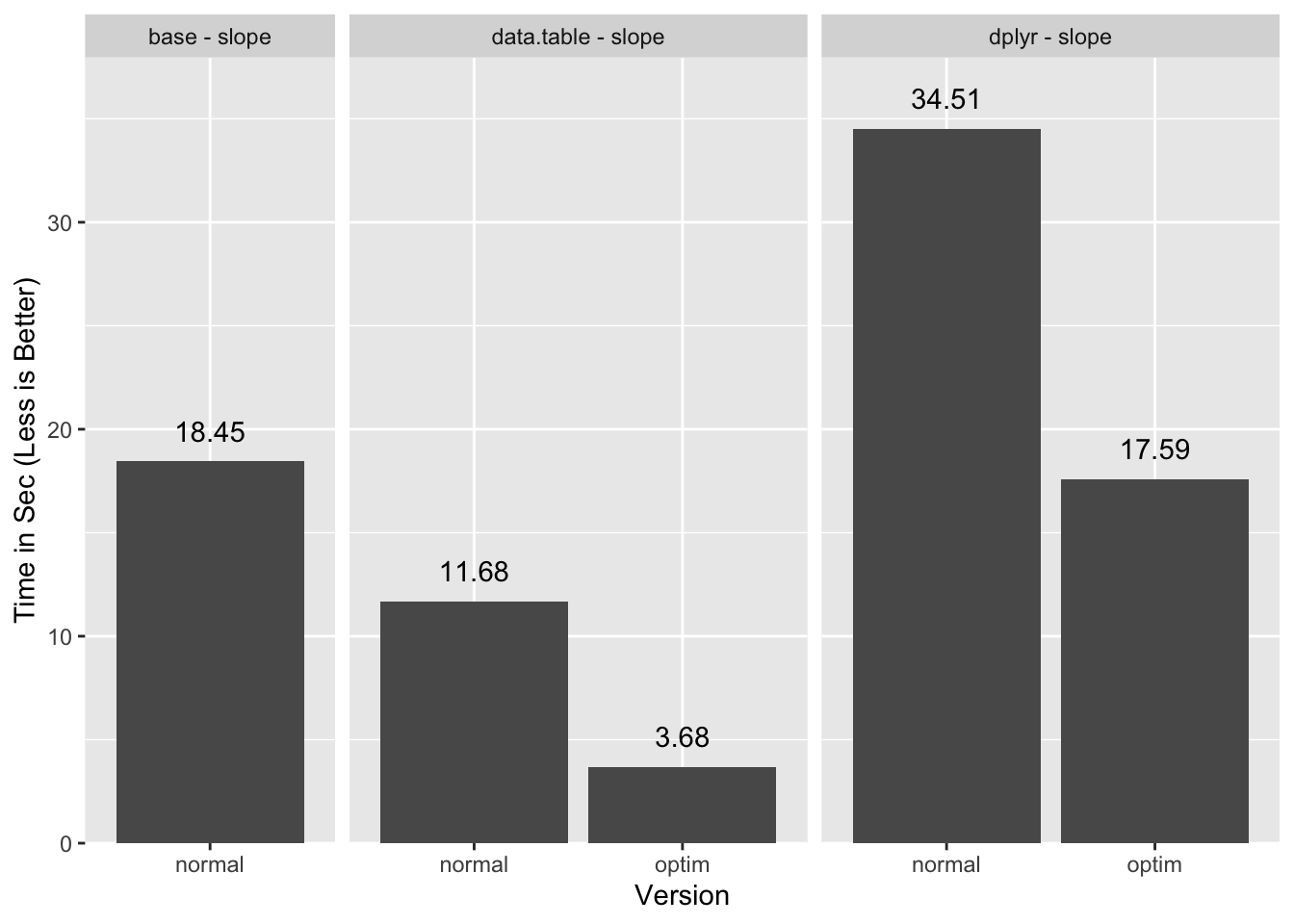
data.table benefits a lot more from enabling “GForce” because the group management portion of the execution is small. Since dplyr is less efficient with groups it does not benefit as much, and for this particular task ends up barely faster than base.

Certainly this test with many groups and few values per group punishes systems that manage groups and joins with any inefficiency. The data.table team has produced a broader set of benchmarks that you can refer to for some idea of performance for dplyr and data.table under different circumstances.

I should point out that “Hybrid Evaluation” is better than “GForce” at respecting the semantics of the calls. For example, dplyr checks that symbols that look like the base summary functions such as mean actually reference those functions. If you do things like mean <- i_am_not_the_mean, dplyr will recognize this and fall back to standard evaluation. Alternatively, if you use mean2 <- base::mean, dplyr will still use “Hybrid Evaluation”. Finally, if a data column actually has a class attribute, dplyr will fall back to standard eval and let dispatch occur. data.table does not handle those cases correctly. This is unlikely to be an issue in typical use cases, but I do like the attention to detail the dplyr team applied here.

Conclusions

With a little thought and care we were able to squeeze out some extra performance out of the super optimized data.table package. While a 2-3x performance improvement may not warrant the work required to get it in day-to-day usage, it could come in handy in circumstances where the optimization is written once and re-used over and over.

Appendix

sessionInfo()

R version 3.5.2 (2018-12-20)
Platform: x86_64-apple-darwin15.6.0 (64-bit)
Running under: macOS High Sierra 10.13.6

Matrix products: default
BLAS: /Library/Frameworks/R.framework/Versions/3.5/Resources/lib/libRblas.0.dylib
LAPACK: /Library/Frameworks/R.framework/Versions/3.5/Resources/lib/libRlapack.dylib

locale:
[1] en_US.UTF-8/en_US.UTF-8/en_US.UTF-8/C/en_US.UTF-8/en_US.UTF-8

attached base packages:
[1] stats     graphics  grDevices utils     datasets  methods   base

other attached packages:
[1] dplyr_0.8.0.1     data.table_1.12.0 ggplot2_3.1.0

loaded via a namespace (and not attached):
 [1] Rcpp_1.0.0       magrittr_1.5     devtools_1.13.6  tidyselect_0.2.5
 [5] munsell_0.5.0    colorspace_1.3-2 R6_2.3.0         rlang_0.3.1
 [9] fansi_0.4.0      plyr_1.8.4       tools_3.5.2      grid_3.5.2
[13] gtable_0.2.0     utf8_1.1.4       cli_1.0.1        withr_2.1.2
[17] lazyeval_0.2.1   digest_0.6.18    assertthat_0.2.0 tibble_2.0.1
[21] crayon_1.3.4     purrr_0.2.5      memoise_1.1.0    glue_1.3.0
[25] compiler_3.5.2   pillar_1.3.1     scales_1.0.0     pkgconfig_2.0.2

DT <- data.table(grp, x, y)
DT[, `:=`(ux=mean(x), uy=mean(y)), keyby=grp]
DT[, `:=`(x_ux=x - ux, y_uy=y - uy)]
DT[, `:=`(x_ux.y_uy=x_ux * y_uy, x_ux2=x_ux^2)]
DTsum <- DT[, .(x_ux.y_uy=sum(x_ux.y_uy), x_ux2=sum(x_ux2)), keyby=grp]
res.slope.dt3 <- DTsum[, .(grp, x_ux.y_uy/x_ux2)]

all.equal(res.slope.base, res.slope.dt3[[2]], check.attributes=FALSE)

[1] TRUE

DT[, `:=`(ux=mean(x), uy=mean(y)), keyby=grp]

DT <- data.table(grp, x, y)
system.time({
  DT[, `:=`(ux=mean(x), uy=mean(y)), keyby=grp]
  DT[, `:=`(x_ux=x - ux, y_uy=y - uy)]
  DT[, `:=`(x_ux.y_uy=x_ux * y_uy, x_ux2=x_ux^2)]
  DTsum <- DT[, .(x_ux.y_uy=sum(x_ux.y_uy), x_ux2=sum(x_ux2)), keyby=grp]
  res.slope.dt2 <- DTsum[, .(grp, x_ux.y_uy/x_ux2)]
})

   user  system elapsed
  7.749   0.335   8.143

system.time({
  res.dplyr3 <- TB %>%
    group_by(grp) %>%
    mutate(ux=mean(x), uy=mean(y)) %>%
    ungroup %>%
    mutate(x_ux=x - ux, y_uy=y - uy, x_ux.y_uy = x_ux * y_uy, x_ux2 = x_ux^2) %>%
    group_by(grp) %>%
    summarize(sx_ux.y_uy=sum(x_ux.y_uy), sx_ux2=sum(x_ux2)) %>%
    ungroup %>%
    mutate(slope= sx_ux.y_uy / sx_ux2) %>%
    select(grp, slope)
})

   user  system elapsed
  30.00    1.03   31.71

DT <- data.table(grp, x, y)
DT.g <- DT[, .(ux=mean(x), uy=mean(y)), keyby=grp]

system.time({
  setkey(DT, grp)
  DT[DT.g]
})

   user  system elapsed
  2.305   0.169   2.496

TB <- tibble(grp, x, y)
TB.g <- TB %>% group_by(grp) %>% summarise(ux=mean(x), uy=mean(y))
system.time(TB %>% inner_join(TB.g))

   user  system elapsed
  4.888   0.471   5.836

system.time({
  res.dplyr3 <- TB %>%
    group_by(grp) %>%
    summarize(ux=mean(x), uy=mean(y)) %>%
    inner_join(TB, ., by='grp') %>%
    mutate(x_ux=x-ux, y_uy=y-uy, x_ux.y_uy=x_ux*y_uy, x_ux2=x_ux^2) %>%
    group_by(grp) %>%
    summarize(x_ux.y_uy=sum(x_ux.y_uy), x_ux2=sum(x_ux2)) %>%
    ungroup %>%
    mutate(slope=x_ux.y_uy / x_ux2) %>%
    select(grp, slope)
})

   user  system elapsed
  26.07    1.45   28.34

all.equal(res.slope.base, res.dplyr3[[2]], check.attributes=FALSE)

[1] TRUE