In One Corner…

As we saw in our Faster Group Statistics post, data.table is the
heavyweight champ in the field. Its gforce functions and fast grouping put it
head and shoulders above all challengers. And yet, here we are, about to throw
our hat in the ring with nothing but base R functionality. Are we out of our
minds?
Obviously I wouldn’t be writing this if I didn’t think we had a chance,
although the only reason we have a chance is because data.table generously
contributed its fast radix sort to R 3.3.0. Perhaps it is ungracious of
us to use it to try to beat data.table, but where’s the fun in being gracious?
The Ring, and a Warmup
Ten million observations, ~one million groups, no holds barred:
RNGversion("3.5.2"); set.seed(42)
n     <- 1e7
n.grp <- 1e6
grp   <- sample(n.grp, n, replace=TRUE)
noise <- rep(c(.001, -.001), n/2)  # more on this later
x     <- runif(n) + noise
y     <- runif(n) + noise          # we'll use this later
Let’s do a warm-up run, with a simple statistic. We use vapply/split
instead of tapply as that will allow us to work with more complex statistics
later. sys.time is a wrapper around system.time that runs the expression
eleven times and returns the median timing. It is defined in the
appendix.
sys.time({
  grp.dat <- split(x, grp)
  x.ref <- vapply(grp.dat, sum, 0)
})
user system elapsed
6.235 0.076 6.316Let’s repeat by ordering the data first because pixie dust:
sys.time({
  o <- order(grp)
  go <- grp[o]
  xo <- x[o]

  grp.dat <- split(xo, go)
  xgo.sum <- vapply(grp.dat, sum, numeric(1))
})
user system elapsed
2.743 0.092 2.840 And now with data.table:
library(data.table)
DT <- data.table(grp, x)
setDTthreads(1)             # turn off multi-threading
sys.time(x.dt <- DT[, sum(x), keyby=grp][[2]])
user system elapsed
0.941 0.030 0.973Ouch. Even without multithreading data.table crushes even the ordered
split/vapply. We use one thread for more stable and comparable results.
We’ll show some multi-threaded benchmarks at the end.
Interlude - Better Living Through Sorted Data
Pixie dust is awesome, but there is an even more important reason to like sorted
data: it opens up possibilities for better algorithms. unique makes for a
good illustration. Let’s start with a simple run:
sys.time(u0 <- unique(grp)) user system elapsed
1.223 0.055 1.290We are ~40% faster if we order first, including the time to order1:
sys.time({
  o <- order(grp)
  go <- grp[o]
  u1 <- unique(go)
})
user system elapsed
0.884 0.049 0.937identical(sort(u0), u1)[1] TRUEThe interesting thing is that once the data is ordered we don’t even need to use
unique and its inefficient hash table. For example, in:
(go.hd <- head(go, 30)) [1] 1 1 1 1 1 1 1 1 1 1 1 2 2 2 2 2 2 2 3 3 3 3 3 3 3 4 4 4 4 4We just need to find the positions where the values change to find the unique
values, which we can do with diff, or the
slightly-faster-for-this-purpose2:
go[-1L] != go[-length(go)]It is clear looking at the vectors side by side that the groups change when they are not equal (showing first 30):
go[-1L]         : 1 1 1 1 1 1 1 1 1 1 2 2 2 2 2 2 2 3 3 3 3 3 3 3 4 4 4 4 4
go[-length(go)] : 1 1 1 1 1 1 1 1 1 1 1 2 2 2 2 2 2 2 3 3 3 3 3 3 3 4 4 4 4
To get the unique values we can just use the above to index into go, though we
must offset by one element:
sys.time({
  o <- order(grp)
  go <- grp[o]
  u2 <- go[c(TRUE, go[-1L] != go[-length(go)])]
})
user system elapsed
0.652 0.017 0.672identical(u1, u2)[1] TRUESame result, but twice the speed of the original, again including the time to order. Most of the time is spent ordering as we can see by how quickly we pick out the unique values once the data is ordered:
sys.time(u2 <- go[c(TRUE, go[-1L] != go[-length(go)])]) user system elapsed
0.135 0.016 0.151The main point I’m trying to make here is that it is a big deal that order
is fast enough that we can switch the algorithms we use downstream and get an
even bigger performance improvement.
A big thank you to team
data.tablefor sharing the pixie dust.
Group Sums
It’s cute that we can use our newfound power to find unique values, but can we
do something more sophisticated? It turns out we can. John Mount, shows
how to compute group sums using cumsum on group-ordered
data3. With a little work we can generalize it.
The concept is to order by group, compute cumulative sum, pull out the last value for each group, and take their differences. Visually:
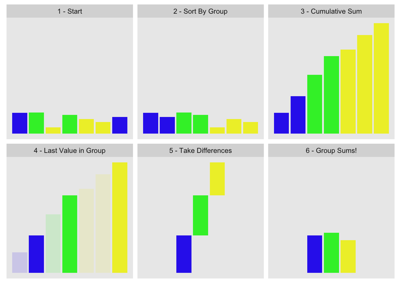
This is the data we used for the visualization:
g1[1] 1 2 3 2 3 3 1x1[1] 0.915 0.937 0.286 0.830 0.642 0.519 0.737The first three steps are obvious:
ord <- order(g1)
go <- g1[ord]
xo <- x1[ord]
xc <- cumsum(xo)
Picking the last value from each group is a little harder, but we can do so with
the help of base::rle. rle returns the lengths of repeated-value
sequences within a vector. In a vector of ordered group ids, we can use it to
compute the lengths of each group:
go[1] 1 1 2 2 3 3 3grle <- rle(go)
(gn <- grle[['lengths']])[1] 2 2 3This tells us the first group has two elements, the
second also two, and the last three. We can translate this into indices of the
original vector with cumsum, and use it to pull out the relevant values from
the cumulative sum of the x values:
(gnc <- cumsum(gn))[1] 2 4 7(xc.last <- xc[gnc])[1] 1.65 3.42 4.87To finish we just take the differences:
diff(c(0, xc.last))[1] 1.65 1.77 1.45I wrapped the whole thing into the group_sum function you can
see in the appendix:
group_sum(x1, g1) 1 2 3
1.65 1.77 1.45 Every step of group_sum is internally vectorized4, so the function is
fast. We demonstrate here with the original 10MM data set:
sys.time(x.grpsum <- group_sum(x, grp)) user system elapsed
1.098 0.244 1.344all.equal(x.grpsum, c(x.ref), check.attributes=FALSE)[1] TRUEdata.table is still faster, but we’re within striking distance. Besides, the
real fight is up ahead.
Before we go on, I should note that R provides
base::rowsum, not to be confused with its better known cousin
base::rowSums. And why would you confuse them? Clearly the capitalization
and pluralization provide stark semantic clues that distinguish them like dawn
does night and day. Anyhow…, rowsum is the only base R function I know of
that computes group statistics with arbitrary group sizes directly in compiled
code. If all we’re trying to do is group sums, then we’re better off using that
instead of our homegrown cumsum version:
sys.time({
  o <- order(grp)
  x.rs <- rowsum(x[o], grp[o], reorder=FALSE)
})
user system elapsed
1.283 0.105 1.430all.equal(x.grpsum, c(x.rs), check.attributes=FALSE)[1] TRUEA summary of timings so far:
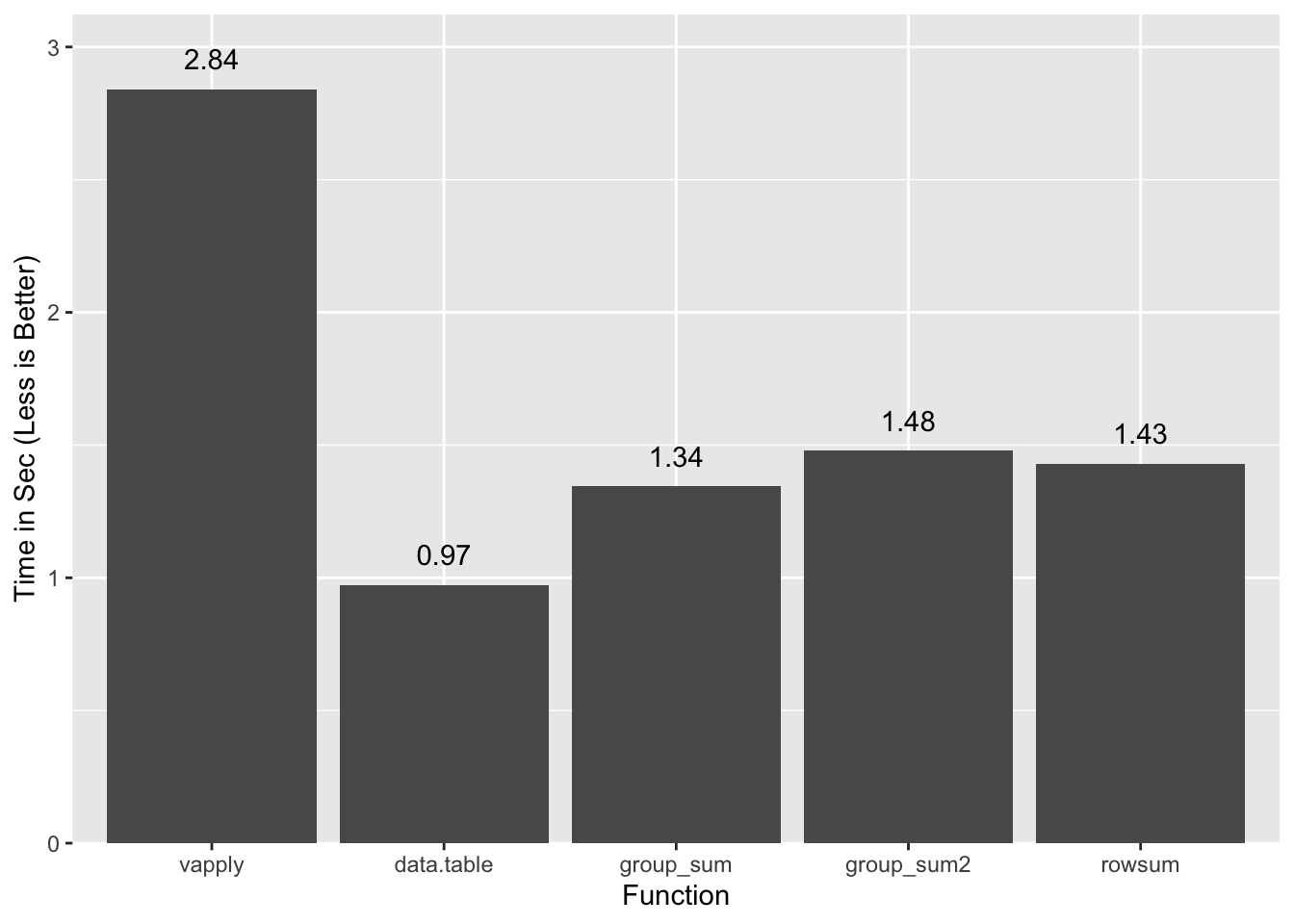
vapply/split and rowsum use ordered inputs and include the time to order
them. data.table is single thread, and
group_sum2 is a version of
group_sum that handles NAs and infinite values. Since performance is
comparable for group_sum2 we will ignore the NA/Inf wrinkle going forward.
So You Think You Can Group-Stat?
Okay, great, we can sum quickly in base R. One measly stat. What good is that if we want to compute something more complex like the slope of a bivariate regression, as we did in our prior post? As a refresher this is what the calculation looks like:
\[\frac{\sum(x_i - \bar{x})(y_i - \bar{y})}{\sum(x_i - \bar{x})^{2}}\]
The R equivalent is5:
slope <- function(x, y) {
  x_ux <- x - mean.default(x)
  y_uy <- y - mean.default(y)
  sum(x_ux * y_uy) / sum(x_ux ^ 2)
}
We can see that sum shows up explicitly, and somewhat implicitly via
mean6. There are many statistics that essentially boil down to
adding things together, so we can use group_sum (or in this case its simpler
form .group_sum_int) as the wedge to breach the barrier to fast grouped
statistics in R:
.group_sum_int <- function(x, last.in.group) {
  xgc <- cumsum(x)[last.in.group]
  diff(c(0, xgc))
}
group_slope <- function(x, y, grp) {
  ## order inputs by group
  o <- order(grp)
  go <- grp[o]
  xo <- x[o]
  yo <- y[o]

  ## group sizes and group indices
  grle <- rle(go)
  gn <- grle[['lengths']]
  gnc <- cumsum(gn)              # Last index in each group
  gi <- rep(seq_along(gn), gn)   # Group recycle indices

  ## compute mean(x) and mean(y), and recycle them
  ## to each element of `x` and `y`:
  sx <- .group_sum_int(xo, gnc)
  ux <- (sx/gn)[gi]
  sy <- .group_sum_int(yo, gnc)
  uy <- (sy/gn)[gi]

  ## (x - mean(x)) and (y - mean(y))
  x_ux <- xo - ux
  y_uy <- yo - uy

  ## Slopes!
  x_ux.y_uy <- .group_sum_int(x_ux * y_uy, gnc)
  x_ux2 <- .group_sum_int(x_ux ^ 2, gnc)
  setNames(x_ux.y_uy / x_ux2, grle[['values']])
}
The non-obvious steps involve gn, gnc, and gi. As we saw
earlier with group_sum gn corresponds to how many elements
there are in each group, and gnc to the index of the last element in each
group. Let’s illustrate with some toy values:
(xo <- 2:6) # some values[1] 2 3 4 5 6(go <- c(3, 3, 5, 5, 5)) # their groups[1] 3 3 5 5 5(gn <- rle(go)[['lengths']]) # the size of the groups[1] 2 3(gnc <- cumsum(gn)) # index of last item in each group[1] 2 5Since these are the same quantities used by group_sum, we can use a
simpler version .group_sum_int that takes the index of the last element in
each group as an input:
(sx <- .group_sum_int(xo, gnc)) # group sum[1] 5 15We re-use gnc four times throughout the calculation, which is a big deal
because that is the slow step in the computation. With
the group sums we can derive the $\bar{x}$ values:
(sx/gn) # mean of each group[1] 2.5 5.0But we need to compute $x - \bar{x}$, which means we need to recycle each
group’s $\bar{x}$ value for each $x$. This is what gi does:
(gi <- rep(seq_along(gn), gn))[1] 1 1 2 2 2cbind(x=xo, ux=(sx/gn)[gi], g=go) # cbind to show relationship b/w values x ux g
[1,] 2 2.5 3
[2,] 3 2.5 3
[3,] 4 5.0 5
[4,] 5 5.0 5
[5,] 6 5.0 5For each original $x$ value, we have associated the corresponding $\bar{x}$
value. We compute uy the same way as ux, and once we have those two values
the rest of the calculation is straightforward.
While this is quite a bit of work, the results are remarkable:
sys.time(slope.gs <- group_slope(x, y, grp)) user system elapsed
1.794 0.486 2.312 Compare to the hand-optimized version of data.table from one of our
earlier posts:
sys.time({
  DT <- data.table(x, y, grp)
  setkey(DT, grp)
  DTsum <- DT[, .(ux=mean(x), uy=mean(y)), keyby=grp]
  DT[DTsum, `:=`(x_ux=x - ux, y_uy=y - uy)]
  DT[, `:=`(x_ux.y_uy=x_ux * y_uy, x_ux2=x_ux^2)]
  DTsum <- DT[, .(x_ux.y_uy=sum(x_ux.y_uy), x_ux2=sum(x_ux2)), keyby=grp]
  slope.dt <- DTsum[, .(grp, V1=x_ux.y_uy / x_ux2)]
})
user system elapsed
2.721 0.412 3.139 Oh snap, we’re ~30% faster than data.table! And this is the painstakingly
optimized version of it that computes on groups directly in C code without the
per-group R evaluation overhead. We’re ~3x faster than the straight
“out-of-the-box” version DT[, slope(x, y), grp].
A summary of all the timings:
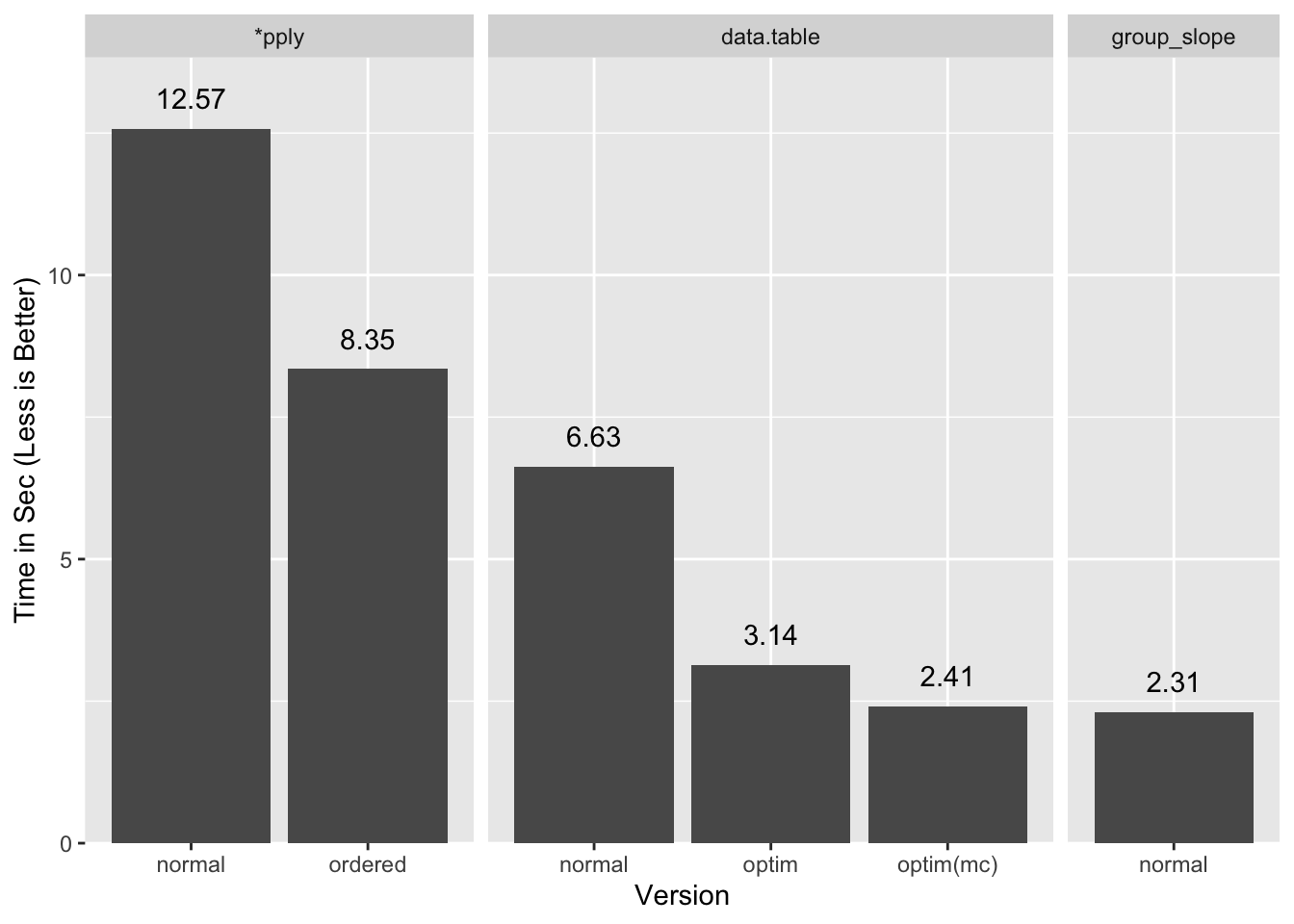
If I let data.table use both my cores it comes close to our timings
(optim(mc)), and presumably would do a little better still with more cores,
but a tie or a slight win for a multi-thread process over a single thread one is
a loss in my books.
More details for the benchmarks are in the appendix.
UPDATE: Michael Chirico points out that it is possible to
reformulate the slope equation into a more favorable form, and under that
form data.table is faster (although our methods are close). I’ll defer
analysis of how generalizable this is to another post, but in the meantime you
can see those benchmarks in the appendix.
Controversy
As we bask in the glory of this upset we notice a hubbub around the judges table. A representative of the Commission on Precise Statics, gesticulating, points angrily at us. Oops. It turns out that our blazing fast benchmark hero is cutting some corners:
all.equal(slope.gs, slope.dt$V1, check.attributes=FALSE)[1] "Mean relative difference: 0.0001161377"cor(slope.dt$V1, slope.gs, use='complete.obs')[1] 0.9999882The answers are almost the same, but not exactly. Our cumsum approach is
exhausting the precision available in double precision numerics. We could
remedy this by using a rowsums based group_slope, but that would
be slower as we would not be able to re-use the group index
data.
Oh, so close. We put up a good fight, but CoPS is unforgiving and we are disqualified.
Conclusions
We learned how we can use ordered data to our advantage, and did something quite
remarkable in the process: beat data.table at its own game, but for a
technicality. Granted, this was for a more complex statistic. We will never be
able to beat data.table for simple statistics with built-in gforce
counterparts (e.g. sum, median, etc.), but as soon as we step away from
those we have a chance, and even for those we are competitive7.
In Part 3 of the Hydra Chronicles we will explore why we’re running into precision issues and whether we can redeem ourselves (hint: we can).
Appendix
Acknowledgments
- John Mount, for the initial
cumsumidea. - Michael Chirico for the clever alternate formulation to slope, and for having the time and patience to remind me of the expected value forms and manipulations of variance and covariance.
- Dirk Eddelbuettel for copy edit suggestions.
- Matt Dowle and the other
data.tableauthors for contributing the radix sort to R. - Hadley Wickham and the
ggplot2authors forggplot2with which I made the plots in this post.
Image Credits
- Rock-em, 2009, by Ariel Waldman, under CC BY-SA 2.0, cropped.
Updates
- 2019-06-10:
- Slope reformulation.
- Included missing
sys.timedefinition. - Bad links.
- 2019-06-11: session info.
- 2019-06-12: fix covariance formula.
Session Info
sessionInfo()R version 3.6.0 (2019-04-26)
Platform: x86_64-apple-darwin15.6.0 (64-bit)
Running under: macOS Mojave 10.14.5
Matrix products: default
BLAS: /Library/Frameworks/R.framework/Versions/3.6/Resources/lib/libRblas.0.dylib
LAPACK: /Library/Frameworks/R.framework/Versions/3.6/Resources/lib/libRlapack.dylib
locale:
[1] en_US.UTF-8/en_US.UTF-8/en_US.UTF-8/C/en_US.UTF-8/en_US.UTF-8
attached base packages:
[1] stats graphics grDevices utils datasets methods base
other attached packages:
[1] data.table_1.12.2sys.time
sys.time <- function(exp, reps=11) {
  res <- matrix(0, reps, 5)
  time.call <- quote(system.time({NULL}))
  time.call[[2]][[2]] <- substitute(exp)
  gc()
  for(i in seq_len(reps)) {
    res[i,] <- eval(time.call, parent.frame())
  }
  structure(res, class='proc_time2')
}
print.proc_time2 <- function(x, ...) {
  print(
    structure(
      x[order(x[,3]),][floor(nrow(x)/2),],
      names=c("user.self", "sys.self", "elapsed", "user.child", "sys.child"),
      class='proc_time'
) ) }
Reusing Last Index
The key advantage group_slope has is that it can re-use gnc, the vector of
indices to the last value in each group. Computing gnc is the expensive part
of the cumsum group sum calculation:
o <- order(grp)
go <- grp[o]
xo <- x[o]
sys.time({
  gn <- rle(go)[['lengths']]
  gi <- rep(seq_along(gn), gn)
  gnc <- cumsum(gn)
})
user system elapsed
0.398 0.134 0.535Once we have gnc the group sum is blazing fast:
sys.time(.group_sum_int(xo, gnc)) user system elapsed
0.042 0.008 0.050Other Slope Benchmarks
vapply
Normal:
sys.time({
  id <- seq_along(grp)
  id.split <- split(id, grp)
  slope.ply <- vapply(id.split, function(id) slope(x[id], y[id]), 0)
})
user system elapsed
12.416 0.142 12.573all.equal(slope.ply, c(slope.rs), check.attributes=FALSE)[1] TRUESorted version:
sys.time({
  o <- order(grp)
  go <- grp[o]
  id <- seq_along(grp)[o]
  id.split <- split(id, go)
  slope.ply2 <- vapply(id.split, function(id) slope(x[id], y[id]), 0)
})
user system elapsed
8.233 0.105 8.351 all.equal(slope.ply2, c(slope.rs), check.attributes=FALSE)[1] TRUEdata.table
Normal:
setDTthreads(1)
DT <- data.table(grp, x, y)
sys.time(DT[, slope(x, y), grp])
user system elapsed
6.509 0.066 6.627 Normal multi-thread:
setDTthreads(0)
DT <- data.table(grp, x, y)
sys.time(DT[, slope(x, y), grp])
user system elapsed
7.979 0.112 6.130 Optimized:
library(data.table)
setDTthreads(1)
sys.time({
  DT <- data.table(grp, x, y)
  setkey(DT, grp)
  DTsum <- DT[, .(ux=mean(x), uy=mean(y)), keyby=grp]
  DT[DTsum, `:=`(x_ux=x - ux, y_uy=y - uy)]
  DT[, `:=`(x_ux.y_uy=x_ux * y_uy, x_ux2=x_ux^2)]
  DTsum <- DT[, .(x_ux.y_uy=sum(x_ux.y_uy), x_ux2=sum(x_ux2)), keyby=grp]
  res.slope.dt2 <- DTsum[, .(grp, V1=x_ux.y_uy / x_ux2)]
})
user system elapsed
2.721 0.412 3.139 Optimized multi-core:
setDTthreads(0)
sys.time({
  DT <- data.table(grp, x, y)
  setkey(DT, grp)
  DTsum <- DT[, .(ux=mean(x), uy=mean(y)), keyby=grp]
  DT[DTsum, `:=`(x_ux=x - ux, y_uy=y - uy)]
  DT[, `:=`(x_ux.y_uy=x_ux * y_uy, x_ux2=x_ux^2)]
  DTsum <- DT[, .(x_ux.y_uy=sum(x_ux.y_uy), x_ux2=sum(x_ux2)), keyby=grp]
  res.slope.dt2 <- DTsum[, .(grp, V1=x_ux.y_uy / x_ux2)]
})
user system elapsed
5.332 0.842 2.412 Reformulated Slope
Special thanks to Michael Chirico for providing this alternative formulation to the slope calculation:
\[ \begin{matrix} Slope& = &\frac{\sum(x_i - \bar{x})(y_i - \bar{y})}{\sum(x_i - \bar{x})^{2}}\\ & = &\frac{Cov(x, y)}{Var(x)}\\\ & = &\frac{E[(x - E[x])(y - E[y])]}{E[(x - E[x])^2]}\\\ & = &\frac{E[xy] - E[x]E[y]}{E[x^2] - E[x]^2} \end{matrix} \]
Where we take E[...] to signify mean(...). See the Wikipedia pages for
Variance and Covariance for the step-by-step simplifications of
the expected value expressions.
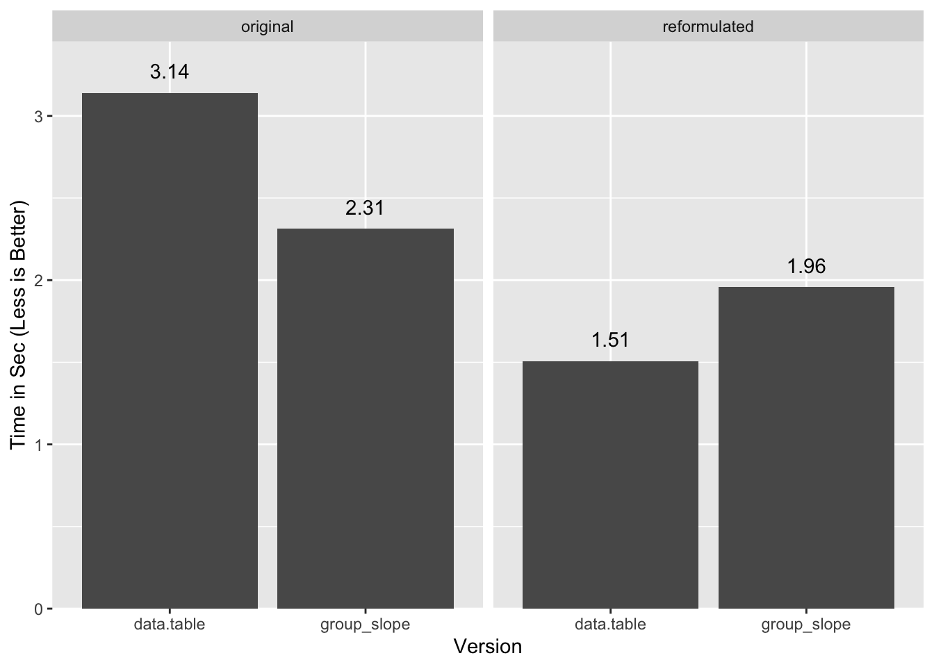
A key feature of this formulation is there is no interaction between grouped statistics and ungrouped as in the original. This saves the costly merge step and results in a substantially faster calculation (single thread):
sys.time({
  DT <- data.table(x, y, xy=x*y, x2=x^2, grp)
  slope.dt.re <- DT[,
    .(ux=mean(x), uy=mean(y), uxy=mean(xy), ux2=mean(x2)),
    keyby=grp
  ][,
    setNames((uxy - ux*uy)/(ux2 - ux^2), grp)
  ]
})
user system elapsed
1.377 0.126 1.507But careful as there are precision issues here too, as warned on the variance page:
This equation should not be used for computations using floating point arithmetic because it suffers from catastrophic cancellation if the two components of the equation are similar in magnitude. There exist numerically stable alternatives.
We observe this to a small extent by comparing to our vapply based
calculation:
quantile(slope.ply2 - slope.dt.re, na.rm=TRUE) 0% 25% 50% 75% 100%
-6.211681e-04 -4.996004e-16 0.000000e+00 4.996004e-16 1.651546e-06 We can apply a similar reformulation to group_slope:
group_slope_re <- function(x, y, grp) {
  o <- order(grp)
  go <- grp[o]
  xo <- x[o]
  yo <- y[o]

  grle <- rle(go)
  gn <- grle[['lengths']]
  gnc <- cumsum(gn)              # Last index in each group

  ux <- .group_sum_int(xo, gnc)/gn
  uy <- .group_sum_int(yo, gnc)/gn
  uxy <- .group_sum_int(xo * yo, gnc)/gn
  ux2 <- .group_sum_int(xo^2, gnc)/gn

  setNames((uxy - ux * uy)/(ux2 - ux^2), grle[['values']])
}
sys.time(slope.gs.re <- group_slope_re(x, y, grp))
user system elapsed
1.548 0.399 1.957 In this case data.table flips the advantage:
Function Definitions
group_sum
group_sum <- function(x, grp) {
  ## Order groups and values
  ord <- order(grp)
  go <- grp[ord]
  xo <- x[ord]

  ## Last values
  grle <- rle(go)
  gnc <- cumsum(grle[['lengths']])
  xc <- cumsum(xo)
  xc.last <- xc[gnc]

  ## Take diffs and return
  gs <- diff(c(0, xc.last))
  setNames(gs, grle[['values']])
}
Cumulative Group Sum With NA and Inf
A correct implementation of the single pass cumsum based group_sum requires
a bit of work to handle both NA and Inf values. Both of these need to be
pulled out of the data ahead of the cumulative step otherwise they would wreck
all subsequent calculations. The rub is they need to be re-injected into the
results, and with Inf we need to account for groups computing to Inf,
-Inf, and even NaN.
I implemented a version of group_sum that handles these for illustrative
purposes. It is lightly tested so you should not consider it to be generally
robust. We ignore the possibility of NAs in grp, although that is something
that should be handled too as rle treats each NA value as distinct.
group_sum2 <- function(x, grp, na.rm=FALSE) {
  if(length(x) != length(grp)) stop("Unequal length args")
  if(!(is.atomic(x) && is.atomic(y))) stop("Non-atomic args")
  if(anyNA(grp)) stop("NA vals not supported in `grp`")

  ord <- order(grp)
  grp.ord <- grp[ord]
  grp.rle <- rle(grp.ord)
  grp.rle.c <- cumsum(grp.rle[['lengths']])
  x.ord <- x[ord]

  # NA and Inf handling. Checking inf makes this 5% slower, but
  # doesn't seem worth adding special handling for cases w/o Infs

  has.na <- anyNA(x)
  if(has.na) {
    na.x <- which(is.na(x.ord))
    x.ord[na.x] <- 0
  } else na.x <- integer()
  inf.x <- which(is.infinite(x.ord))
  any.inf <- length(inf.x) > 0
  if(any.inf) {
    inf.vals <- x.ord[inf.x]
    x.ord[inf.x] <- 0
  }
  x.grp.c <- cumsum(x.ord)[grp.rle.c]
  x.grp.c[-1L] <- x.grp.c[-1L] - x.grp.c[-length(x.grp.c)]

  # Re-inject NAs and Infs as needed

  if(any.inf) {
    inf.grps <- findInterval(inf.x, grp.rle.c, left.open=TRUE) + 1L
    inf.rle <- rle(inf.grps)
    inf.res <- rep(Inf, length(inf.rle[['lengths']]))
    inf.neg <- inf.vals < 0

    # If more than one Inf val in group, need to make sure we don't have
    # Infs of different signs as those add up to NaN
    if(any(inf.long <- (inf.rle[['lengths']] > 1L))) {
      inf.pos.g <- group_sum2(!inf.neg, inf.grps)
      inf.neg.g <- group_sum2(inf.neg, inf.grps)
      inf.res[inf.neg.g > 0] <- -Inf
      inf.res[inf.pos.g & inf.neg.g] <- NaN
    } else {
      inf.res[inf.neg] <- -Inf
    }
    x.grp.c[inf.rle[['values']]] <- inf.res
  }
  if(!na.rm && has.na)
    x.grp.c[findInterval(na.x, grp.rle.c, left.open=TRUE) + 1L] <- NA

  structure(x.grp.c, groups=grp.rle[['values']], n=grp.rle[['lengths']])
}
sys.time(x.grpsum2 <- group_sum2(x, grp))
user system elapsed
1.147 0.323 1.479 all.equal(x.grpsum, x.grpsum2)[1] TRUEFor more details on why the hash table based
uniqueis affected by ordering see the pixie dust post.↩Additional logic will be required for handling NAs.↩
I did some light research but did not find other obvious uses of this method. Since this approach was not really practical until
data.tableradix sorting was added to base R in version 3.3.0, its plausible it is somewhat rare. Send me links if there are other examples.↩R code that carries out looped operations over vectors in compiled code rather than in R-level code.↩
This is a slightly modified version of the original from prior post that is faster because it uses
mean.defaultinstead ofmean.↩mean(x)in R is not exactly equivalent tosum(x) / length(x)becausemeanhas a two pass precision improvement algorithm.↩We leave it as an exercise to the reader to implement a fast
group_medianfunction.↩