In Which It Dawns On Me That I Know Nothing
It wasn’t supposed to be this way. You shouldn’t be looking at drawing of a Lernean Hydra laughing its ass off. This post was going to be short, sweet, and useful. Instead it turned into a many-headed monster that is smugly sitting on my chest smothering me. What follows here is a retelling of my flailing attempt at chopping off one of its heads.
It all started on a lark to see if I could make base R competitive with the
undisputed champ data.table at computing group statistics. That thought
alone is scoff-worthy enough that I deserve little sympathy for how
off-the-rails this whole thing has gone1.
TL;DR: ordering data can have a huge impact on how quickly it can be processed because of micro-architectural factors such as cache, out-of-order execution, and branch prediction. Yes, even in R.
Let’s skip back to the care-free, hydra-less days on twitter when I should have known better than to post:
A great example of #FOSS at work: #rdatatable team’s contributes their radix sort to #rstats. ~50x faster ordering in this e.g.
This type of improvement on such a fundamental operation is invaluable (more on this next week). Thank you @MattDowle @arun_sriniv
“More on this next week”… 🤣🤣🤣. Aaaah, what a fool. That was almost three months ago. The key observations back then were that:
data.tablecontributed its radix sort to R in R3.3.0, and as a resultorderbecame 50x faster under some work loads.
I was also alluding to something fairly remarkable that happens when you order data before you process it. Let’s illustrate with 10MM items in ~1MM groups:
RNGversion("3.5.2"); set.seed(42)
n     <- 1e7
n.grp <- 1e6
grp   <- sample(n.grp, n, replace=TRUE)
x     <- runif(n)
The first step for computing group statistics is to split the data by group:
gs <- split(x, grp)
str(head(gs, 3))  # display structure of first 3 groups
List of 3
$ 1: num [1:11] 0.216 0.537 0.849 0.847 0.347 ...
$ 2: num [1:7] 0.0724 0.1365 0.5364 0.0517 0.1887 ...
$ 3: num [1:7] 0.842 0.323 0.325 0.49 0.342 ...split breaks up our vector x into a list of vectors defined by grp. We
can see above the structure of the first three of these vectors. This is a slow
step in group statistic computations, so lets time it with sys.time (a wrapper
around system.time2):
sys.time(gs <- split(x, grp)) user system elapsed
5.643 0.056 5.704Compare to what happens if we order the inputs first:
sys.time({
  o <- order(grp)
  xo <- x[o]
  go <- grp[o]
  gso <- split(xo, go)
})
user system elapsed
1.973 0.060 2.054Sorting values by group prior to running split makes it over twice as fast,
including the time required to sort the data. We just doubled the speed of
an important workhorse R function without touching the code. And we get the
exact same results:
identical(gs, gso)[1] TRUEPixie dust. data.table pixie dust.
Disclaimer: I have no special knowledge of microarchitecture other than what I learned while researching this post. I cannot guarantee the accuracy of all the details herein, but the broad outlines should be mostly correct and are backed by experimentation. I only hope that my relative inexperience on the topic makes my writing on it more accessible.
Latency Is The Enemy
Something is going on underneath the hood that dramatically affects the performance of the random scenario. The fundamental problem is that main memory (RAM) access is laggy. Over the past few decades CPU processing speed has grown faster than memory latency has dropped. Nowadays it may take ~200 CPU cycles to have a CPU data request fulfilled from main memory.
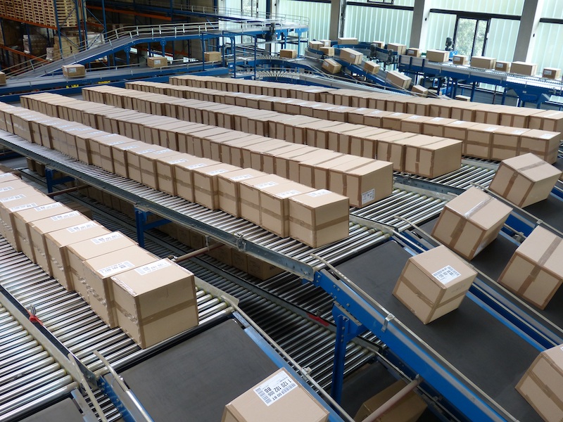
Main memory latency is terrible, but thankfully its bandwidth has kept pace with processor speeds. A useful analogy is that of a long conveyor belt connecting a storage warehouse (main memory) to its factory (CPU). The first item requested from the warehouse will be slow to arrive (latency), but if the conveyor belt is loaded efficiently it will keep the factory fully supplied from the moment the first item arrives (bandwidth).
This analogy can give us some idea of the type of problems caused by random inputs. Suppose the factory places a request for items from the warehouse, taking care to order the items in the request form. This is what the request will look like mid-process, with processed items in yellow:
                                   | WAREHOUSE
  ---------------------------------+-----------------------
  < < < < < < 📦📦📦📦< < < < 📦📦📦📦< < < < 📦< < < < <
  ---------------------------------+-----------------------
                                   |           👷
  Request:                         | FP   TZ   GZ   FT   YJ
  FP FT GZ TZ YJ                   | 📦 | 📦 | 📦 | 📦 | 📦
  FP FT GZ TZ YJ                   | 📦 | 📦 | 📦 | 📦 | 📦
  FP FT GZ TZ YJ                   | ⬜ | 📦 | 📦 | ⬜ | 📦
  FP FT GZ TZ YJ                   | ⬜ | 📦 | 📦 | ⬜ | 📦
                                   | ⬜ | 📦 | 📦 | ⬜ | 📦
                                   | ⬜ | 📦 | ⬜ | ⬜ | 📦
It takes time for the worker to change stations. So long as packages are requested repeatedly from the same station the worker can fully utilize the conveyor belt. As soon as they need to change stations, there will be a gap in the conveyor belt corresponding to the time it takes to do so. Unsurprisingly when the items are requested randomly the ratio of package to gaps is worse:
                                   | WAREHOUSE
  ---------------------------------+-----------------------
  < < < < < < 📦< < < < 📦< < < < 📦< < < < 📦< < < < < <
  ---------------------------------+-----------------------
                                   |           👷
  Request:                         | FP   TZ   GZ   FT   YJ
  FT YJ TZ YJ FP                   | 📦 | 📦 | 📦 | 📦 | 📦
  TZ FT YJ GZ GZ                   | 📦 | 📦 | 📦 | 📦 | 📦
  FP TZ FT TZ GZ                   | 📦 | 📦 | 📦 | 📦 | 📦
  GZ FP YJ FP FT                   | 📦 | 📦 | 📦 | 📦 | 📦
                                   | 📦 | 📦 | 📦 | 📦 | 📦
                                   | ⬜ | ⬜ | ⬜ | ⬜ | 📦
While this analogy only bears a passing resemblance to some parts of what happens in the memory system, the concept applies generally. Anytime you have high latency and high bandwidth, predictable requests will utilize bandwidth much better than unpredictable ones.
Microarchitecture To The Rescue?
Chip designers have engaged in micro-architectural heroics to conceal main memory latency. Microarchitecture is The Implementation Detail. Higher level programs like C are compiled into machine instructions. In simpler times, machines would just follow those instructions. Nowadays a CPU only pretends to do that. “Behind the scenes” out of sight of the program it re-interprets them in whatever way it sees fit3. The key constraint is that the CPU state visible to the program must be consistent with the instructions, but that leaves room for some hair raising optimizations. Everything that happens “behind the scenes” is the microarchitecture.
There are two main classes of microarchitectural tricks used to mask main memory latency. The first one involves interpreting instructions in such a way that the conveyor belt can be kept fully utilized (i.e. few gaps) after the first item is requested. This includes preloading memory areas the CPU is likely to need based on prior access patterns, executing operations out-of-order so that memory requests for later operations are initiated while earlier ones wait for theirs to be fulfilled, speculating at which conditional branch will be executed before its condition is known so that out-of-order execution can continue past the branch, and other optimizations.
The second involves having some amount of low latency memory known as cache. In our conveyor belt analogy it might be a shelf next to the assembly station with room for a few items. When items can be retrieved from cache we are insulated from main memory latency. Cache is very limited because it requires a more expensive design and it must be close to the CPU, typically on the exclusive real estate of the CPU die:
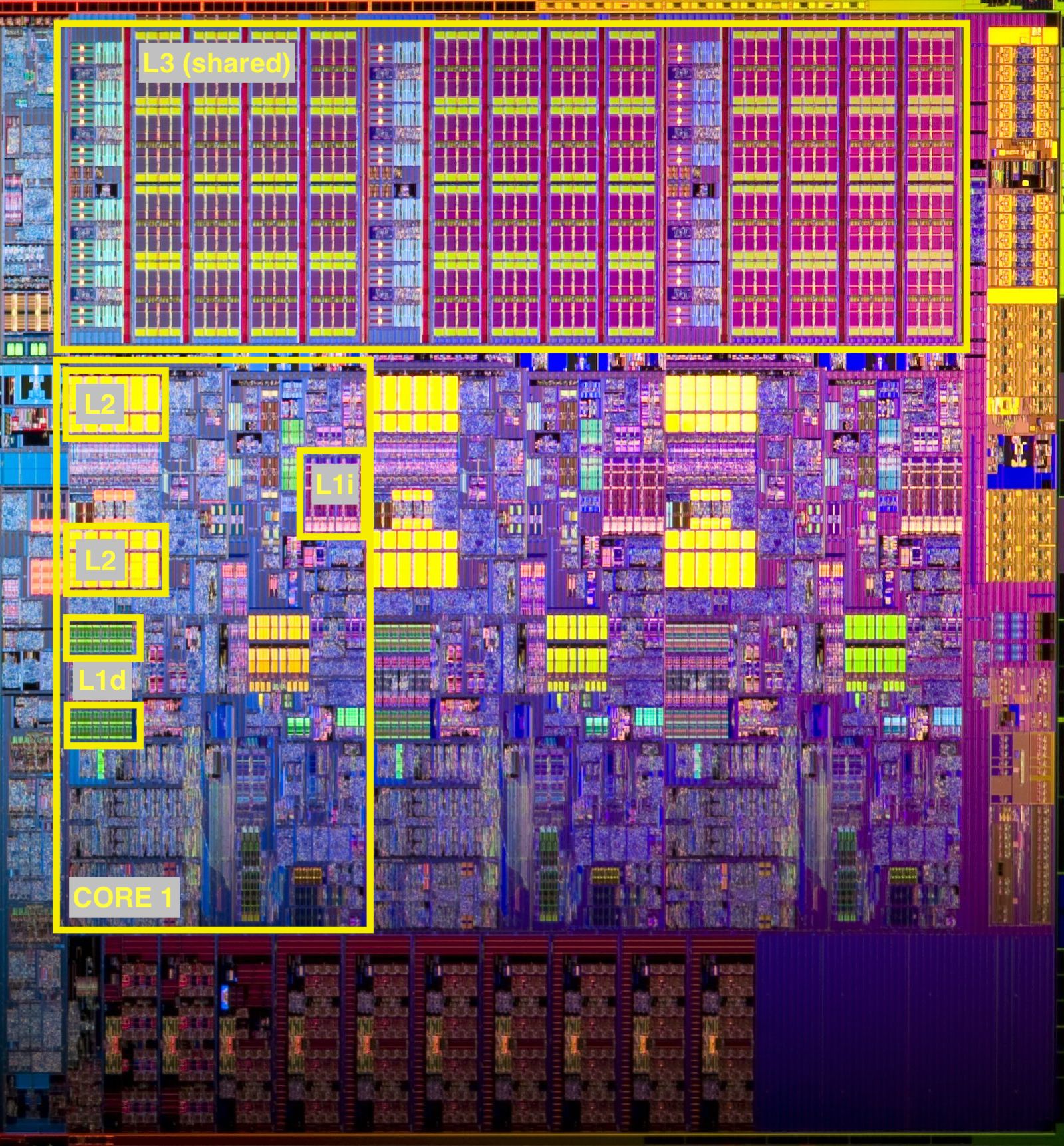
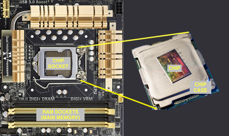
We can see three levels of cache labeled L1, L2, and L34, with the first two inside the cores, and the last shared across all cores. Each core will have its own L1 and L2 cache, though we only label them within one core. L1 cache is split between data cache (L1d) and instruction cache (L1i). You can get a sense of how different cache and main memory are by looking at the bigger picture. Main memory is on a different continent:
In many cases the combination of these tricks is sufficient to conceal or at
least amortize the latency over many accesses, but there are pathological
memory access patterns that defeat them. splitting the randomly ordered
vector is an example of this. treeprof gives us detailed timings for
the random and sorted split calls5:
times in milliseconds
                                         random  |      sorted
split --------------------------- : 7239 -    0  |  1573 -   0
    split.default --------------- : 7239 - 1997  |  1573 - 137
        as.factor --------------- : 5242 - 2471  |  1436 - 630
            sort ---------------- : 2771 -    0  |   806 -   0
                unique.default -- : 2705 - 2705  |   789 - 789
                sort.default ---- :   67 -    0  |    17 -   0
                    sort.int ---- :   67 -   27  |    17 -   7
                        order --- :   40 -   40  |     9 -   9
There are many differences between the two runs, but let’s focus on the highlighted numbers to start. These correspond to the internal C code that scans through the input vector and the normalized group vectors6, and copies each input value into the result vector indicated by the group7. The code will take the same exact number of steps irrespective of input order, yet there is a ~15x speed-up between the sorted (137ms) and randomized versions (1,997ms).
Modelling Cache Effects
Ideally we would keep our whole working set in cache and not have to worry about
main memory latency. Unfortunately the working set is often larger than cache.
We’re interested in exploring how cache and working set size affect the speed of
the split.default calculation.
My system has a three level cache hierarchy as in the pictured die8. Each level is larger but slower than the previous one9:
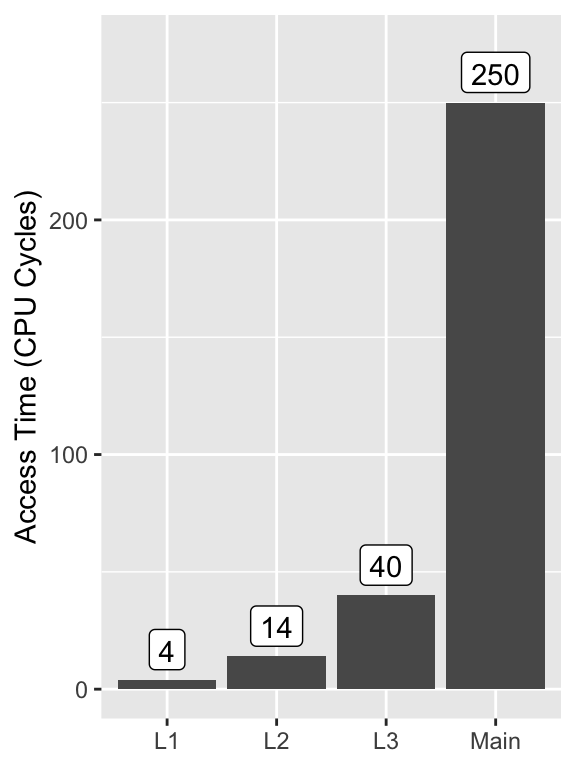
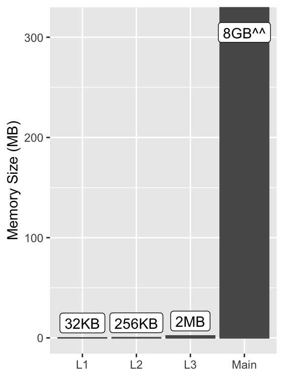
On a CPU clocked at 1.2GHz like mine a 4 cycle L1 access will take ~3.3ns and a 250 cycle main memory access will take ~200ns.
One way to explore the cache effects is to build a model of what we think memory access times should be based on working set size and the above data. If cache is effective we would expect processing times to follow our model. We show our current working set size (10MM elements) as a vertical dashed line10, the modeled access times as colored lines, and observed timings as dots:
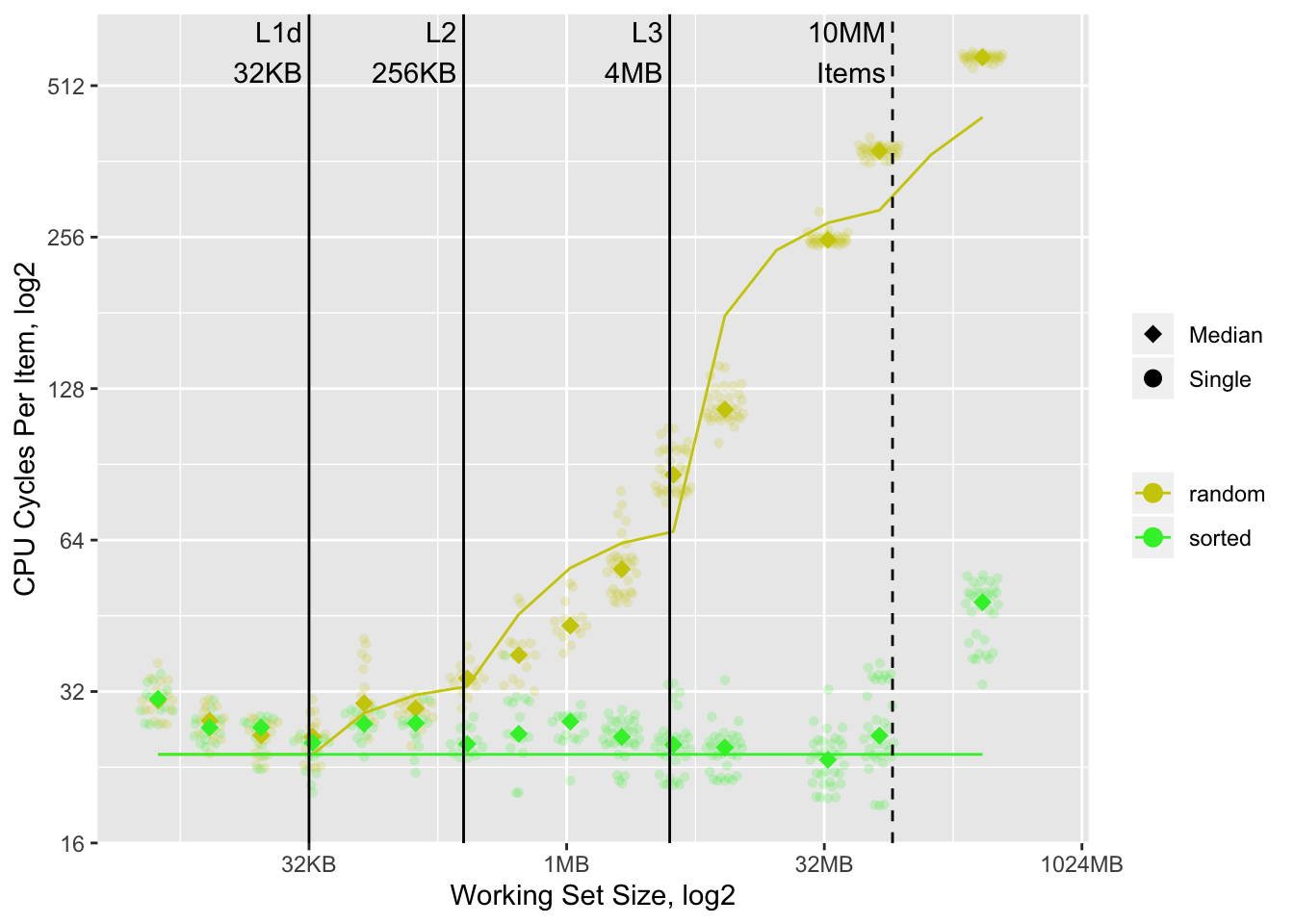
Outside of a few anomalies11 the model works remarkably well. It predicts a ~13x slowdown in the random vs. sorted case for the 10MM element working set, which is close to the observed ~15x. It is reasonably accurate for most other working set sizes.
split.default has six memory accesses12 per element
processed13. When the inputs are ordered all of them are
sequential. When they are not two of those are no longer sequential.
Sequential access are simple and predictable, and as a result memory systems have built-in optimizations for them such as prefetching14 and stream buffers15 (these are both forms of speculative execution16). We assume sequential accesses can be met at L1 cache speeds without consuming cache. Conversely random accesses do not benefit from these optimizations. We assume they are subject to the full memory system latency, the magnitude of which will vary depending on how much of the working set fits in each level of cache. Transitions to a slower level of memory manifest as an increase in per-element time that asymptotically17 approaches the slower memory’s latency18.
The implementation of this cache model is available in the appendix.
Since we are only modeling cache effects and the timings line up so closely, this implies that there are no other optimizations for random accesses in effect19. Cache does mitigate the cost of random accesses, but its effect quickly dissipates as working set size increases.
Degrees of Pathology
We now have a reasonable understanding of why split.default works much faster
with ordered than unordered input. What is not explained is why the combination
of ordering the inputs and splitting them is faster than splitting them
directly. After all the ordering process itself involves random memory
accesses:
o <- order(grp)
go <- grp[o]            # random access
xo <- x[o]              # random access
split.default(xo, go)   # sequential
Even ignoring the order call, the indexing steps required to order x and
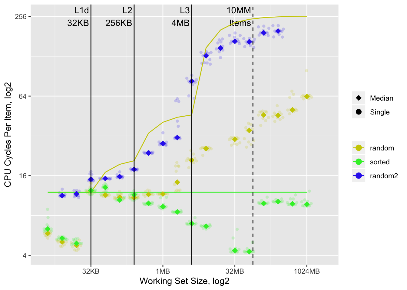
grp into xo and go are random accesses. I ran the timings for x[o]
as well as for a version with x and o pre-sorted, and superimposed them with
a cache-only model for those accesses:
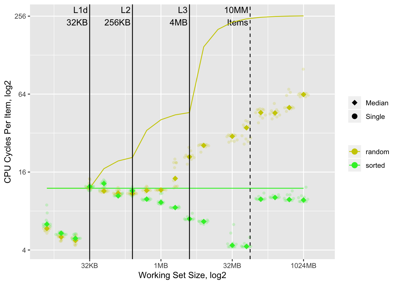
There are many interesting things going on20, but the most notable one is that the random case substantially outperforms the corresponding cache-only model.
Let’s examine what the subset C code is doing, shown here in pseudo R guise:
res <- numeric(length(grp))
seqi <- seq_along(grp)
for(i in seqi) {
  val <- x[i]        # sequential - fetch x value to copy
  idx <- o[i]        # sequential - fetch write offset
  res[idx] <- val    # random - write x value at offset
}
The slow step is res[idx] <- val as idx can point to any location in the
result vector. But the nice thing about this loop is that each iteration is
independent of all others. This allows the processor to begin execution of
multiple loop iterations without waiting for the first one to complete,
i.e. out-of-order.
Out-of-order instructions are kept “in-flight” in the reorder buffer21, an on-die memory structure that can store a number of both pending and complete instructions. The purpose of the buffer is to allow instructions to be executed out-of-order, but have their results committed in logical program order. Once a result is committed it becomes part of the CPU state visible to the program.
Let’s pretend our system’s reorder buffer supports up to eight “instructions”
“in-flight”. We can recast the first two iterations of the previous for
loop into the following instructions pseudo R code
instructions22:
## loop iteration 1
i1        <- seqi[1]               # PENDING
val1      <- x[i1]                 # PENDING
idx1      <- o[i1]                 # PENDING
res[idx1] <- val1                  # PENDING
## loop iteration 2
i2        <- seqi[2]               # PENDING
val2      <- x[i2]                 # PENDING
idx2      <- o[i2]                 # PENDING
res[idx2] <- val2                  # PENDING
We renamed the i, val, and idx variables by appending the loop number to
each of them23. This allows the CPU to re-order them without
instructions from later iterations overwriting earlier ones. They can now be
executed in the following order:
i1        <- seqi[1]               # PENDING
i2        <- seqi[2]               # PENDING

val1      <- x[i1]                 # PENDING
val2      <- x[i2]                 # PENDING

idx1      <- o[i1]                 # PENDING
idx2      <- o[i2]                 # PENDING

res[idx1] <- val1                  # PENDING
res[idx2] <- val2                  # PENDING
The processor is free to chose any instruction to execute that does not depend
on others. In this case both the i1 and i2 instructions are eligible, so
the processor could execute one, the other, or even both
simultaneously24. Shortly after the first main memory access
is complete this will be the state:
## i1     <- seqi[1]               # retired
i2        <- seqi[2]               # complete
i3        <- seqi[3]               # PENDING

val1      <- x[i1]                 # PENDING
val2      <- x[i2]                 # PENDING

idx1      <- o[i1]                 # PENDING
idx2      <- o[i2]                 # PENDING

res[idx1] <- val1                  # PENDING
res[idx2] <- val2 # PENDINGi1, and i2 are both computed. Additionally, the i1 instruction is retired,
meaning its result is visible to the program and it no longer occupies one of
the eight “in-flight” slots. The i2 instruction cannot be retired despite
being complete because in the logical flow of the program it comes after the
val1, idx1, and res[idx1] commands that are still pending. The i3
instruction takes up the slot freed by the retirement of the i1 instruction.
The same dynamic will play out for the val* and idx* steps, which will lead
to:
## i1     <- seqi[1]               # retired
## val1   <-   x[i1]               # retired
## idx1   <-   o[i1]               # retired

i2        <- seqi[2]               # complete
i3        <- seqi[3]               # complete

val2      <- x[i2]                 # complete
val3      <- x[i3]                 # complete

idx2      <- o[i2]                 # complete
idx3      <- o[i3]                 # complete

res[idx1] <- val1                  # PENDING
res[idx2] <- val2                  # PENDING
This is where out-of-order execution really shines. All prior memory accesses
are sequential, so executing out-of-order is of marginal value as subsequent
reads would be fast anyway. But the writes to res are random and
subject to the full memory latency. Out-of-order execution allows us to run
them both concurrently. This is of value because main memory has substantial
parallelism built-in25, i.e. the warehouse has multiple workers
available to load (or unload) the conveyor belt. Processing speed for this type
of access will grow with the degree of main memory parallelism and the size of
the “in-flight” instruction window26.
One way to confirm that out-of-order execution is in play is to prevent it in an otherwise similar workload by adding a sequential loop dependency. We can use “chasing indices” like this one:
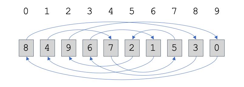
Each vector element contains in it the (0-based) index of the next element to
visit. The arrows illustrate the path that results from following the indices.
Unfortunately it isn’t possible to do this efficiently in pure R code, so
instead I wrote a C function to do it, and superimposed its
timings on the previous ones as the blue random2 data set:
With the sequential dependency timings are back in line with the theoretical cache-only model, demonstrating that the random subset likely benefited from out-of-order execution.
Sure enough, it turns out that the split.default code has a sequential
dependency in it too: it uses an offset vector to track where in each group
vector to write the next value, and this vector is updated in the
loop27.
Random accesses are pathological to modern memory systems, but those with sequential dependencies are downright killer. When we order our input vectors first we isolate random accesses to simple operations without sequential dependencies and give the memory system the best chance to mitigate latency.
Branch Prediction
One optimization we glossed over is branch prediction. An out-of-order CPU
cannot put instructions “in-flight” past a branch (e.g. if statement) that
depends on incomplete previous instructions because it does not know which side
of the branch to put “in-flight”. Modern CPUs will make an educated guess and
speculate about which instructions to put “in-flight” so it can maintain the
benefits of out-of-order execution when it guesses right.
Ironically the key feature of branch predicting CPUs is not the ability to guess, but rather the ability to recover from an incorrect guess. The reorder buffer assists in this by marking all “in-flight” operations predicated on a branch guess as speculative. These may then be discarded if the guess is discovered to be incorrect when the branch condition computation completes. Mispredictions do have a cost (15-20 cycles on my system28), so CPU designers invest a substantial amount of effort to improve branch prediction.
Branch prediction likely only plays a minor role in our examples29;
however, for completeness sake I’ve contrived a new one that demonstrates its
effect. Compilers are notoriously aggressive at removing branches, so for
controlled testing I wrote a toy example in C and compiled it with all
optimizations turned off (-O0):
SEXP add_walk2(SEXP x) {
  R_xlen_t size = XLENGTH(x);
  int *x_ptr=INTEGER(x);
  int accum = 0;

  for(R_xlen_t i = 0; i < size; ++i) {
    if(*x_ptr > 0) {accum++;} else {accum--;}  // BRANCH
    ++x_ptr;
  }
  return ScalarInteger(accum);
}
This function computes the sum of a logical vector interpreting TRUE values as
+1 and FALSE values as -1. We can test it with logical vectors with
varying proportions of TRUE values, both random and sorted:
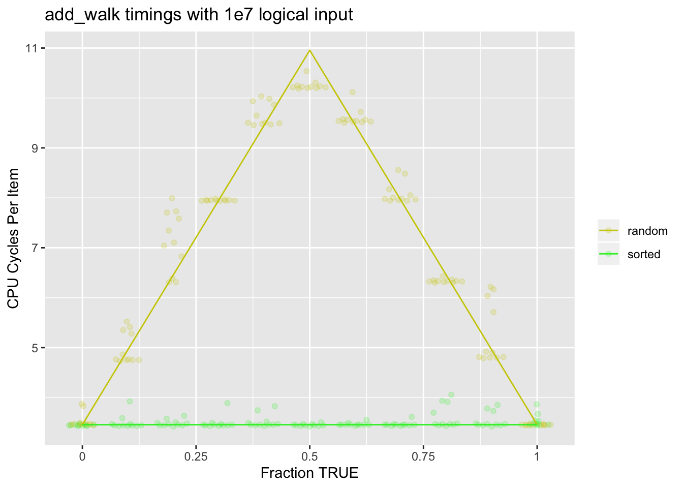
The colored branch misprediction penalty model lines use 15 cycles penalty per misprediction, which fits the observed timings well. In the randomly ordered case the branch predictor cannot do better than predicting the higher frequency branch on average. In the sorted case there is essentially no misprediction penalty as predicting recently seen branch directions is a good strategy.
A 15-20 cycle misprediction penalty is likely a best case scenario. If the mispredictions interfered with main memory accesses instead of register-only operations as above, the cost would be much higher.
A Faustian Bargain

So much ingenuity has gone into designing and implementing modern memory systems that it’s easy to forget the whole thing is a massive hack. Case in point: a raft of severe processor security vulnerabilities published over the past two years that exploit micro-architectural optimizations.
The limitations of the microarchitecture expose its supposedly hidden implementation details to probing via observation of timings. The expense of the silicon that implements it has led to it being shared concurrently across processes. The combination of these makes for a horror show of severe and difficult to fix vulnerabilities.
MDS (bottom-right in inset) was announced while I was in the process of writing this post, about sixteen months after the Meltdown and Spectre vulnerabilities were disclosed (top row). What’s staggering is that changes that Intel introduced to its newest processors to mitigate Meltdown have made some of the MDS vulnerabilities worse.
My little seguë here has little relevance to the post other than microarchitecture is involved and the timing of the disclosures of the most recent vulnerabilities. If you have been reading the headlines over the past year or so and have wondered exactly what this was all about, I encourage you to read the papers. They are remarkably accessible, and occasionally downright funny.
Loose Ends
The internal code in split.default had the largest proportional difference
between sorted and unsorted cases, but both as.factor and unique.default
together account for a larger part of the overall difference:
times in milliseconds
                                         random  |      sorted
split --------------------------- : 7239 -    0  |  1573 -   0
    split.default --------------- : 7239 - 1997  |  1573 - 137
        as.factor --------------- : 5242 - 2471  |  1436 - 630
            sort ---------------- : 2771 -    0  |   806 -   0
                unique.default -- : 2705 - 2705  |   789 - 789
                sort.default ---- :   67 -    0  |    17 -   0
                    sort.int ---- :   67 -   27  |    17 -   7
                        order --- :   40 -   40  |     9 -   9
These are the steps that turn the groups into factor levels so they can be used
as offsets into the result vector for split.default. Both of them rely on
hash tables: unique uses one to detect whether a value is
duplicated, and as.factor uses one via match to assign a unique
index to each distinct value in its input.
Why is the sorting effect less pronounced with these? Most likely because
hashing by its nature undoes some of the benefits of the sort. In R, hash
tables are stored as vectors twice the size of the vector being
hashed30. So in unique.default(grp), we are generating a
hash table with twenty million elements, of which we will eventually use
~one million31. Worse, from a memory system perspective, the
hashing function will try to distribute the values evenly and randomly
throughout the hash vector. Nothing like large memory allocations accessed
randomly to make the memory system happy.
Sorting the data still helps because for each group the same hash key will be accessed repeatedly such that only the first access for each group is subjected to the full main memory latency, other optimizations notwithstanding.
One last thing to point out: we ordered our vectors once, but we reaped the micro-architectural benefits in three different places. This in part explains how we get so much of a performance improvement even when we account for the time it takes to order the data.
Conclusions
The irony in all this is that the micro-architectural mess we just slogged through is a side-show. The principal reason I care about ordering data is that it opens up possibilities for different and more efficient processing algorithms, independent of micro-architectural factors. It’s just that when I ran into such an in-your-face manifestation of them I could not resist exploring.
Stay tuned for Part II of the Hydra Chronicles, in which we will explore how ordered data can do amazing things. Originally I was planning on ending the post with the hydra drawing minus a couple of heads, but its grown on me and I feel bad doing that. Henceforth it will be a mascot and the name of this series of blog posts, and it won’t make any sense except to those like you that read the first one. That’s okay, it will be our inside joke.
Appendix
Software Acknowledgments
- Matt Dowle and the other
data.tableauthors for contributing the radix sort to R. - Hadley Wickham and the
ggplot2authors forggplot2with which I made the plots in this post. - Oleg Sklyar, Duncan Murdoch, Mike Smith, Dirk Eddelbuettel, Romain Francois,
Karline Soetaert for
inline.
References
Here is the subset of the references I consulted that I found particularly helpful. There are many others linked through the main body of the document and the footnotes.
- Ulrich Drepper, “What Every Programmer Should Know About Memory”, 2007: a comprehensive review of modern memory systems, with an emphasis on main memory and cache.
- Ed Jorgensen, “x86-64 Assembly Language Programming with Ubuntu”, 2019: If you are interested in exploring microarchitecture further, you’ll want at least a very basic understanding of assembly language32. This is a great introduction you can skim through reasonably quickly to get a sense of what’s what.
- R. M. Tomasulo, “An Efficient Algorithm For Exploiting Multiple Arithmetic Units”, 1967: implicitly introduces the concept of register renaming to allow out-of-order execution. Back then memory latency was less of an issue and the main objective was to better utilize the multiple execution units available in the processor. This paper substantially pre-dates the reorder buffer and speculative execution, so out-of-order “retirements” were possible with independent calculations, but out-of-order speculation past branches was not.
- Norman Jouppi, “Improving Direct-Mapped Cache Performance by the Addition of a Small Fully-Associative Cache and Prefetch Buffers”, 1990: introduces the idea of the stream buffer (among other things), which allows fast reads of sequential data without polluting the cache.
- Agner Fog, “The microarchitecture of Intel, AMD and VIA CPUs”, 2018: micro-architectural details of processors starting with the Pentium. Includes characteristics such as the number of reorder buffer entries, cache latency times and organization, and an introduction to micro-architectural concepts.
- Moritz Lipp, etal., “Meltdown: Reading Kernel Memory from User Space”, 2018: Meltdown vulnerability paper includes a useful Background section and gives a good idea of how things can go wrong.
Image Credits
- Hydra With Fedora(s), by Larry Wentzel, under CC BY-NC 2.0, haberdashery and haberdasher removed.
- Conveyor Belt, by unknown, under CC0 Public Domain.
- Westmere 6 Core, posted by redstern, license unknown, in-post version annotated and cropped to three cores, the annotations are derived from those in the Bad Concurrency Post and if those are correct, these should be correct since the Westmere architecture is a shrunken version of the Nehalem.
- Intel 14nm Skylake, by Fritzchens Frits, under CC0 Public Domain, and Asus Motherboard, by Asus PR.
- Meltdown, Spectre, and Foreshadow logos by Natascha Eidl, under CC0 Public Domain.
- MDS logo by Marina Minkin, under CC0 Public Domain.
Function Definitions
sys.time
Please note there is an error in this function. When reps is odd, it returns
the timing of the run just faster than the median run. Since all timings were
taken with this error in effect, they should still be comparable.
sys.time <- function(exp, reps=11) {
  res <- matrix(0, reps, 5)
  time.call <- quote(system.time({NULL}))
  time.call[[2]][[2]] <- substitute(exp)
  gc()
  for(i in seq_len(reps)) {
    res[i,] <- eval(time.call, parent.frame())
  }
  structure(res, class='proc_time2')
}
print.proc_time2 <- function(x, ...) {
  print(
    structure(
      x[order(x[,3]),][floor(nrow(x)/2),],
      names=c("user.self", "sys.self", "elapsed", "user.child", "sys.child"),
      class='proc_time'
) ) }
Cache Model
The implementation of the cache model for the random accesses for
split.default.
test.sizes <- c(9:25)
access.times <- c(4, 14, 40, 250)
mem.sizes <- c(L1=15, L2=18, L3=22, Main=33)

cache_times <- function(set.sizes, mem.sizes, access.times) {
  hit.rates <- outer(
    set.sizes, mem.sizes, function(x, y) 1 - pmax(0, x - y) / x
  )
  times <- matrix(numeric(), nrow=nrow(hit.rates), ncol=ncol(hit.rates))
  mult <- rep(1, nrow(hit.rates))
  for(i in seq_len(ncol(hit.rates))) {
    times[,i] <- hit.rates[,i] * access.times[i] * mult
    mult <- mult * (1 - hit.rates[,i])
  }
  times
}
### Two randomly accessed data sets, the result vector (numeric),
### and the offset vector, integer, and roughly a tenth of the size of the
### result vector since there is one offset per group

set.sizes.1 <- setNames(2^test.sizes * 8, test.sizes)
set.sizes.2 <- setNames(2^test.sizes * 4 / 10, test.sizes)

times1 <- cache_times(set.sizes.1, 2^mem.sizes, access.times)
times2 <- cache_times(set.sizes.2, 2^mem.sizes, access.times)
times <- rowSums(times1) + rowSums(times2)
Index Chasing
Simulate a pointer chasing chain by generating indices that reference the next index to go to. We make the index a numeric rather than an integer just to match working set sizes we used in other examples.
rand_path <- function(size) {
  if(!is.numeric(size) || length(size) != 1 || is.na(size) || size < 1)
    stop("bad input size")
  idx <- sample(as.integer(size - 1L)) + 1
  res <- numeric(size)
  res[c(1, head(idx, -1))] <- idx
  res[tail(idx, 1)] <- 1
  res - 1
}
We can then “walk” these indices with some C code that writes the index values to a new vector in the order of the walk. This is not exactly equivalent to indexing a vector in random order, but the number of random memory accesses is the same and that is the limiting element.
## CAREFUL: `x` should only be as produced by `rand_path`
walkrand <- inline::cfunction(
  sig=c(x='numeric'),
  body="
  R_xlen_t len = XLENGTH(x);
  double *x_ptr = REAL(x);
  SEXP res = PROTECT(allocVector(REALSXP, len));
  double *resvec = REAL(res);
  R_xlen_t idx = 0;

  for(R_xlen_t i = 0; i < len; ++i) {
    idx = x_ptr[idx];
    resvec[i] = idx;
  }
  UNPROTECT(1);
  return res;
")
Branch Prediction
The function is in the body of the post, but due to the need to
compile it with optimizations turned off I had to take special steps to use it.
First I temporarily updated ~/.R/Makevars:
CFLAGS = -S -masm=intel -O0    // For disassembly
CFLAGS = -O0 -Wall -std=gnu99  // For assembly with no optimization
Then in an R session:
tools::Rcmd('shlib add-walk2.c')
dyn.load('add-walk2.so')
.Call('add_walk2', sample(c(TRUE, FALSE), 1e7, rep=TRUE))
Benchmarking Code
This ended up being a bit messy. The code below runs the benchmarks and stores the result as RDSes. The code inline to the post loads the RDSes and displays the data.
### split.default --------------------------------------------------------------

times <- c(
   1e4, 1e4,  1e4,  5e3,   1e3,  1e3, 1e3,  1e2,  1e2,    50,   25,    25,
   10,    5,    3
)
reps <- c(
    11,  11,   11,   11,    11,   11,   5,    5,     5,    5,    5,     5,
     5,   5,    5
)
ns <- rev(ns)
times <- rev(times) * 2
reps <- rep(reps)

res <- vector('list', 0)
for(i in seq_along(ns)) {
  RNGversion("3.5.2"); set.seed(42)
  n <- ns[i]
  x <- runif(n)
  g <- sample(n/10, n, rep=TRUE)
  go <- sort(g)
  gfo <- as.factor(go)
  gf <- as.factor(g)

  writeLines(sprintf('------ %f -------', n))
  time.normal <-
    # sys.time(for(j in seq_len(times[i])) duplicated.default(g))
    sys.time(for(j in seq_len(times[i])) split.default(x, gf), reps=reps[i])
  time.sorted <-
    sys.time(for(j in seq_len(times[i])) split.default(x, gfo), reps=reps[i])
    # sys.time(for(j in seq_len(times[i])) duplicated.default(go))

  res <- append(
    res, list(
      normal=time.normal, sorted=time.sorted, n=n, times=times[i]
  ) )
  print(time.normal)
  print(time.sorted)
}
  # saveRDS(res, ...)

### Index chasing --------------------------------------------------------------

sizes <- 2^(10:25)
times <- pmax(2^24 / sizes, 1)
sizes.sub <- seq_along(sizes) # tail(seq_along(sizes), 3)
samps <- lapply(sizes[sizes.sub], rand_path)
y <- 11

res <- vector('list', 0)
for(i in seq_along(samps)) {
  idx <- sizes.sub[i]
  writeLines(sprintf('------ %f -------', sizes[idx]))
  time.normal <- sys.time(for(j in seq(times[[idx]])) walkrand(samps[[i]]), y)

  # subsequent processing code relied on having sorted vs unsorted data, so
  # that's why we write the same value twice
  res <- append(
    res, list(
      normal=time.normal, sorted=time.normal, n=sizes[[idx]], times=times[idx]
  ) )
  print(time.normal)
}
  # saveRDS(res, ...)

### Branch Predict -------------------------------------------------------------

fractions <- 0:10
vecs <- lapply(
  fractions,
  function(x) {
    trues <- x
    falses <- 10 - x
    sample(c(rep(TRUE, trues), rep(FALSE, falses)), 1e7, rep=TRUE)
  }
)
vecss <- lapply(vecs, sort)
res <- list()
for(i in seq_along(vecs)) {
  writeLines(sprintf('------ %f -------', fractions[[i]]))
  time.normal <- sys.time(for(j in 1:10) .Call('add_walk2', vecs[[i]]))
  time.sorted <- sys.time(for(j in 1:10) .Call('add_walk2', vecss[[i]]))

  res <- append(
    res, list(
      normal=time.normal, sorted=time.sorted,
      n=1, times=10, fraction=fractions[[i]]/10
  ) )
  print(time.normal)
  print(time.sorted)
}
  # saveRDS(res, ...)
The source of this post is nearing two thousand lines and I haven’t even started addressing the question I set out to answer.↩
It runs
system.timeeleven times and returns the median timing. It is defined in the appendix.↩Another way to think about it is that microarchitecture is to assembly instructions as a compiler is to a C program. In both cases a process will interpret a set of instructions (C code, assembly) into a different lower-level set of instructions (assembly, CPU micro-operations). The processes must abide by constraints (a flavor of the C standard, an Instruction Set Architecture), but these are loose enough to allow outrageous re-interpretation. There are few things quite as humbling as learning just enough assembly that you can look at the disassembly of what you thought was a simple C function and realize there is almost no relationship between what you wrote and what the program is doing other than the semantics are the same, assuming no unintended use of undefined behavior. And then there is the whole microarchitectural layer on top of that. Maybe once upon a time C was close to the metal, but nowadays writing in C to be close to the metal is like hanging out in the basement to be closer to the iron core of the planet.↩
These are labeled on a best-efforts basis and may be incorrect.↩
I manually juxtaposed the output of two
treeprofruns.↩Prior to this step the group vector is turned into integer group numbers that match the offset into the result list that the values of a group will be stored in.↩
The timing corresponds to the
.Internalcall that invokes the C code that does the allocation of the result vector and the copying, although the bulk of the time is spent copying . The.Internalcall does not show up in the R profile data used to build thetreeprofoutput because.Internalis both “special” (i.e.typeof(.Internal) == "special", see?Rprof) and a primitive. “special” functions are those that can access their arguments unevaluated. See R Internals for details.↩My system actually has 64KB of L1 cache, but it is split into 32KB of data cache (L1d), and 32KB of instruction cache (L1i).↩
The latency figures are approximate. In particular, the main memory latency may be incorrect. For cache we use the numbers provided in Agner Fog’s “The microarchitecture of Intel, AMD and VIA CPUs”. For L3 we picked a seemingly reasonable number in the provided range.↩
We use for working set size the portion of the data that cannot be accessed sequentially when the input is randomized. This is the size of the result list of vectors which will be a little over 10MM elements each 8 bytes in size, and the offset tracking vector which will be ~1MM elements, each 4 bytes in size. In reality there is more data involved, but because the rest of it are accessed sequentially, their impact on cache utilization is much lower. Additionally, because the offset tracking vector is so much smaller than the main result list we assume that it will not substantively alter the eviction rate of the larger result set, and it will also not be evicted as any part of it is likely to have been accessed more recently than the result set.↩
Two notable anomalies are (1) decreasing times per item for the smaller sets that are possibly a result of R function call overhead being amortized over an increasing number of entries, and (2) a jump up at largest working set sizes for sequential access that could correspond to the Translation Lookaside Buffer being exhausted. This is a cache for translation of virtual to physical memory addresses. The Intel 64 and IA-32 Optimization Reference Manual notes in table 2-9 that there are 32 2/4MB DTLB entries, which would suggest a TLB walk after 64 or 128MB, around the point we see a timing anomaly. We are being sloppy about accounting as the “working set” size we report is just the randomly accessed memory, but presumably the sequentially accessed memory must be mapped by the TLB as well.↩
We are including only the operations used to process the inputs in the main loop. These are: read input value (1), read factor level (2), fetch target vector from result list (3), read offset for target vector (4), write value to target vector at offset (5), and increment offset (6).↩
There are a few other operations involved, such as allocating memory and incrementing offset counters, but these are a small portion of the overall time.↩
When a cache line is fetched, processors will often fetch the subsequent cache line as well. This is called prefetching.↩
Nima Honarmand’s “Memory Prefetching” lecture strongly suggests data streams can be supported without polluting cache (p13,21-22), that is without consuming much of the cache itself. Same with the Paul Wicks “Miss Caches, Victim Caches and Stream Buffers” presentation (p14-15). Both of them are based off of the Jouppi paper. The June 2016 iteration of the “Intel 64 and IA-32 Optimization Reference Manual” references a “Streaming Prefetcher” a.k.a. “Data Cache Unit Prefetcher” (DCU) in section 2.3.5.4 and the “IP Prefetcher” that feed into L1, but their constraints suggest that it might not be the one doing the buffering. An older version of the same manual only mentions the L2 streamers (sections 2.1.5, 2.2.4, 3.7.3, 7.2, 7.6.3), stating that prefetches go into L2. It is also not clear from the Intel docs that the streamers avoid cache pollution via e.g. a buffer. John McAlpin suggests cache lines can be explicitly marked as LRU so they get evicted first; perhaps this is how pollution is avoided without a stream buffer. My observations are consistent with streams being met at L1 speeds without cache pollution, although it could be due to other factors (e.g. accesses are met at L2 speeds, but multiple accesses are done simultaneously).↩
Actions taken by the microarchitecture that anticipate instruction needs to take advantage of microarchitectural parallelism and mitigate latency. These include branch prediction, prefetching, and similar. Although out-of-order execution is not strictly speculative, in modern systems in combination with branch prediction it becomes so anytime it starts executing instructions past speculated branches.↩
Keep in mind that the x-axis is log base 2, so each step corresponds to a doubling of the working set size. After the first step past a cache level transition, only half the working set can be accessed from the faster cache. After two only a quarter, and so on.↩
There are only three transitions from faster to slower memory, yet there are four bumps in the plot. This is because our working set contains two randomly accessed elements: the result list with the double precision vectors that correspond to each group, and an integer vector that tracks the offsets within each group that the next element will be written to. The last bump corresponds to the point at which the offset integer vector outgrows L3 cache. With ten elements per group on average, we will need ~1 million elements in the offset vector to track each group with a 10MM working set size. At 4 bytes an element, that makes for a ~4MB integer vector, which is the size of L3 cache.↩
It is also possible the reality is more complicated and there are offsetting factors cancelling each other out. I have no easy way of knowing that my inferences about what is happening are correct. I’m relying exclusively on the simple model producing reasonable results, and common sense based on the information I have been able to gather. Ideally I would be able to query performance counters to confirm that cache misses can indeed explain the observed timings, but those are hard to access on OS X, and even harder still for code that is run as part of R. One element that is almost undoubtedly influencing performance is Translation Lookaside Buffer (TLB) misses, which I do not model at all.↩
With working set less than L1 in size, it looks like the system can execute all three memory accesses (two loads, one store) simultaneously. This is not entirely surprising given that my Skylake processor has two load data execution units and one store data execution unit. After that point there is a penalty, which is eventually amortized for the sorted set. Because it is amortized eventually this suggests its not a cache penalty. It may be a TLB (Translation Lookaside Buffer) effect, although it seems too early for that to happen as the DTLB supports 64 4KB pages, and with a 32KB working set (
xo), the total memory we’re using is 32KB + 32KB + 16KB (xo+x+o). The next jump at 64MB could be the same DTLB jump we saw earlier.↩Assuming no sequential instruction dependencies, CPUs that can engage in out-of-order execution can get ahead by as many micro-operations as will fit in the re-order buffer. Re-order buffer sizes vary by architecture. On my Skylake system the reorder buffer supports 224 micro-operations (Agner Fog, p149). There are some further limitations on the types of quantities of any single type of operation in the re-order buffer.↩
The eight instructions we show here will likely correspond to substantially more micro-operations, both because they are intended to symbolize assembler instructions and not micro-operations, and also because the actual C implementation of the R code is more complex than the pseudo code indicates.↩
The 1965 Tomasulo Paper implicitly introduced the concept of register renaming that breaks the false dependency that exists when names/registers are re-used and allows increased instruction-level parallelism.↩
Almost all processors nowadays are superscalar, meaning that they have multiple execution units that can compute simultaneously. More recent processors can execute up to eight micro-operations in parallel, although execution units are specialized so it is not possible to have eight arbitrary operations done in parallel.↩
Main memory parallelism arises from it comprising multiple banks that can be accessed independently. It is difficult to get information on exactly how many independently accessible banks my system has, but it seems likely to be at least 16. So long as the random accesses are from different banks they should all be addressable concurrently. Anandtech goes into some detail on memory banks. See this University of Utah CS7810 presentation for some discussion of the parallelism obtained from banks in DRAM memory, and the introduction to the Wikipedia SDRAM page which also mentions banks, interleaving, and pipelining.↩
This assumes the memory locations are in separate banks, which should be the case for most random accesses, although occasionally it won’t be the case.↩
splittracks the offset at which the next value in a group will be written to, and increments that offset each time a value is written. In other words, in order to know where in the result vector a value needs to go, the CPU needs to know how many times previously that group was written to, which is difficult to do without a level of insight into the code the CPU is unlikely to have.↩Agner Fog lists 15-20 cycles for Haswell, Broadwell, and Skylake on p29 of “The microarchitecture of Intel, AMD and VIA CPUs”.↩
There are a few spots where branch prediction is likely happening. First in the loops proper as the break condition is a branch. Since our loops are long, guessing that the loop will continue indefinitely is an easy and effective guess. More importantly, our loops are dominated by the slow random access, so with out-of-order execution the all the other steps can be run quickly, including the loop condition calculation. In this case the branch will not be the bottleneck and value of branch prediction is limited. Another place it comes in is checking that indices are not NA, and finally in the type conditional in
split.default. However, as was the case earlier, the bottlenecks remain the random accesses even if branch prediction is successful. For example, even if we successfully guess that the group-offset value is not NA, we cannot proceed until we get the offset value to write to the group vector. Finally, it is entirely possible that some of the branches in question are being eliminated by the compiler and are not even in the assembly instructions issued to the processor.↩Hash tables used to take up 4x the size of the hashed input, but in 2004 that was switched to 2x. A tidbit I found fascinating is that the R hash tables are open-addressed, meaning that collisions are resolved by walking along the hash vector until an open slot is found instead of appending an element to the end of a linked list or similar. Additionally, it is the index into the vector that is hashed that is stored, no the value itself. This means all vector types can have an integer hash table (or double if using LONG_VECTOR_SUPPORT, which nowadays is probably the default).↩
Even though we’re only using one million elements from the hash table the cache effective size of it will be likely at least 8 times that as memory is always brought into cache in cache-line size, or 64 bytes. In order to bring in one eight byte numeric value from the hashtable, we have to bring in another 56 bytes of mostly unused hash table around it. In many cases it will be even worse as the hardware prefetcher may bring in two cache lines instead of just one.↩
Assembly instructions are low level commands that can be directly interpreted by the CPU. Programs that are not written in assembly are translated into assembly directly by a compiler, or indirectly by mapping program instructions to pre-compiled assembly instructions.↩