Cool, but Not Eye Popping
As I finished the ray shading post, it occurred to me that it would be pretty cool if we could make these awesome 3D-looking reliefs actually 3D, or at least stereoscopic. After all, how hard could it be? We have the elevation data, so some simple trigonometry should allow us to tilt things left, tilt things right, and voilà. So I did that and it looked like garbage.
That would have been the right time to walk away and move on to more productive
things. Instead, I started messing around with rgl (fantastic package),
but I struggled to get it to do exactly what I wanted programmatically. While
trying to understand how rgl reacts to inputs I read up on 3D projections,
and realized that maybe this could all be done outside of rgl.
And so began this quixotic challenge1 to implement an “efficient-enough”2 3D rendering pipeline using base R only. I took notes along the way to share with those who like me are interested, but unlike me have better time management skills. So, come along for a ride through 3D projections, meshes, perspective adjustments, rasterization, and image processing, all in base R3.
DISCLAIMER: I knew nothing about 3D rendering before starting this post, and now I know just enough to be dangerous. Do not look for 3D rendering best practices here. My criteria for using things in this post is: “does it appear to work”.
Volcano!
Our subject today will be the much-loved volcano, a.k.a. Maunga Whau. We are
going to pretend that the Z-values of the volcano matrix are in the same units
as the grid size (i.e. 10m per unit, as per ?volcano). This is obviously not
the case, but the documentation is just ambiguous enough that I feel comfortable
indulging in this minor fraud for dramatic effect. Here is a height-map of
volcano:
xv <- row(volcano)
yv <- col(volcano)
plot_new(xv, yv)
points(x=rescale(xv), y=rescale(yv), col=gray(rescale(volcano)), pch=15)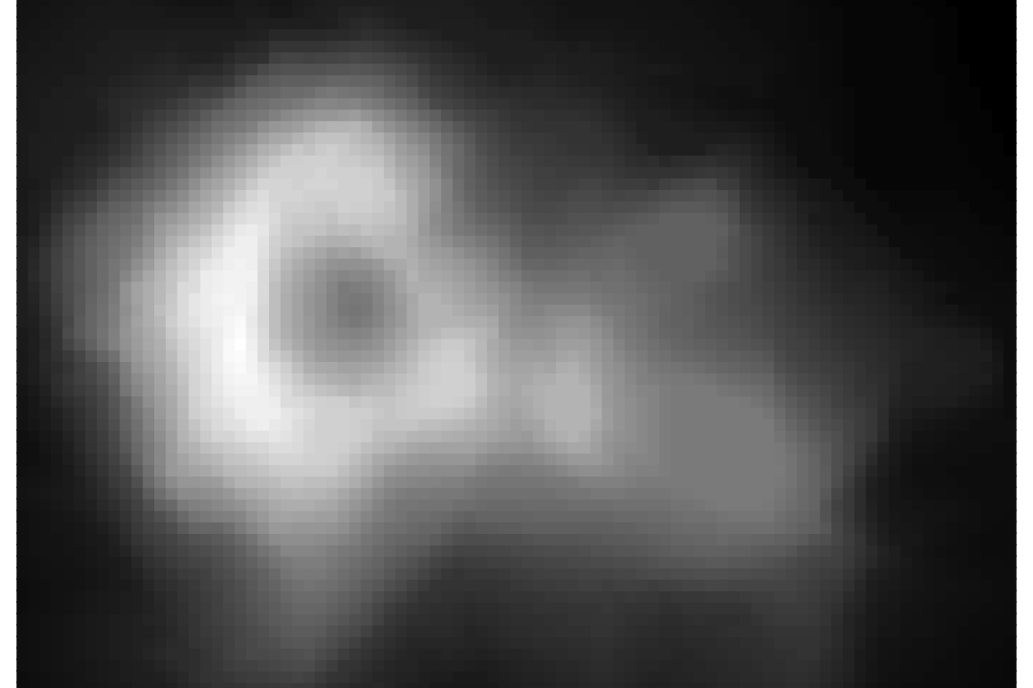
plot_new is a thin wrapper around plot.new that also sets some par
values. rescale rescales values to between zero and one. Both of these are
helper functions defined in the appendix.
As we saw from the ray shading post, it is possible to ray shade elevation maps using base R only. For the sake of exposition I put the code in the shadow demo package, but as far as I’m concerned I’m still abiding by the base-R-only pledge.
library(shadow)
shadow <- ray_shade2(volcano, seq(-90, 90, length=25), sunangle=180)
plot_new(xv, yv)
points(x=rescale(xv), y=rescale(yv), col=gray(shadow), pch=15)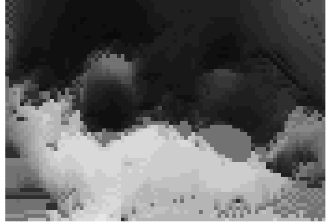
3D Projection
While volcano looks pretty cool from above, we want to provide a more
interesting view. To do this we can use 3D rotation matrices. shadow
implements the rot_* functions, which are thin wrappers that generate the
rotation matrices described in the wikipedia article:
round(rot_z(90), 3) [,1] [,2] [,3]
[1,] 0 -1 0
[2,] 1 0 0
[3,] 0 0 1By our convention the Z-axis is always pointed directly at the user, even after rotations are applied. In other words, it is the model that rotates, not the viewer4. This also means that the X and Y axes remain in their traditional positions.
In order to use the rotation matrix we need our data in long format. This can
be done easily by taking advantage of the row and col functions:
mx.example <- matrix((0:3)*10, nrow=2, ncol=2)
row(mx.example)
[,1] [,2]
[1,] 1 1
[2,] 2 2col(mx.example) [,1] [,2]
[1,] 1 2
[2,] 1 2rbind(x=c(row(mx.example)), y=c(col(mx.example)), z=c(mx.example)) [,1] [,2] [,3] [,4]
x 1 2 1 2
y 1 1 2 2
z 0 10 20 30While this looks rather wide for long format data, I assure you it is long in
spirit. We need it in 3 x n rather n x 3 format for the upcoming matrix
multiplication. As applied to volcano:
volc.l <- rbind(x=c(row(volcano)), y=c(col(volcano)), z=c(volcano))
ncol(volc.l)      # long data has same number of colums ...
[1] 5307length(volcano) # ... as volcano has elements[1] 5307The 3D projection is then just a matrix multiply:
rot <- rot_x(-20) %*% rot_z(65)
volc.lr <- rot %*% volc.l
We need to re-order by Z values to ensure that the nearest points are plotted last so they are not occluded by further points. Recall the Z axis is pointed directly at you, so points with higher Z values are closer.
zord <- order(volc.lr[3,])
vord <- volc.lr[, zord]   # reorder by Z-values
x <- vord[1,]
y <- vord[2,]
plot_new(x, y)
points(rescale(x), rescale(y), col=gray(shadow[zord]), pch=15, cex=0.5)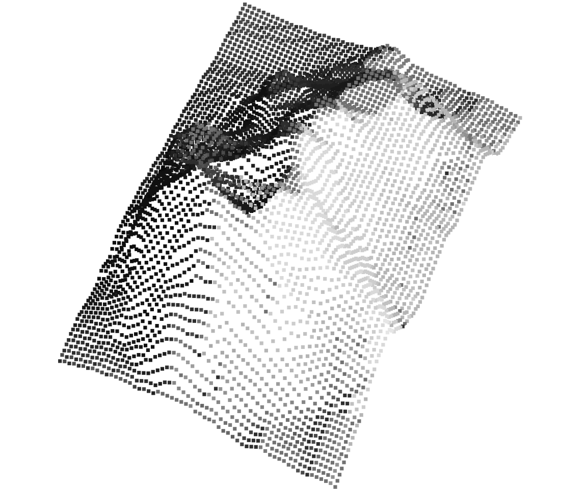
The good news is now we have an awesome looking 3D rendition of our volcano… in the moments after a direct hit from a disruptor cannon.
Interlude I
As you might have guessed one of the reasons why people don’t usually implement 3D rendering pipelines in base R is performance. If we are to have any hope of creating a pipeline that renders things in useful5 time we need to be careful about how we structure our data and calculations.
In an earlier blog post we found that list and list-matrix data structures are often faster to operate on than the pure-vector equivalent matrices and arrays. Here we turn our long volcano matrix into list format:
vl <- lapply(seq_len(nrow(volc.lr)), function(x) volc.lr[x,])
vl <- c(vl, list(shadow))              # add texture info
names(vl) <- c('x', 'y', 'z', 't')     # 't' for texture
str(vl)
List of 4
$ x: num [1:5307] -0.4837 -0.0611 0.3615 0.7842 1.2068 ...
$ y: num [1:5307] 35.5 36.6 37.8 39 40.2 ...
$ z: num [1:5307] 93.5 94.1 94.8 95.4 96 ...
$ t: num [1:87, 1:61] 1 1 1 1 1 1 1 1 1 1 ...Throughout the rest of this blog post we will use techniques explored at length
in the aforementioned post. If you are not familiar with lapply, do.call,
Map, Reduce, and similar functional list manipulation facilities, you should
consider reading that post. We’ll wait for you right here =).
Meshes
Tiles
As our disintegrating volcano demonstrates, we can’t just use elevation data as point coordinates. One possibility is to turn our point “cloud” into a mesh. It turns out that making a mesh out of an arbitrary point cloud is one of those “seems easy but isn’t” problems. Worse, the typical implementations involve some kind of sequential process that is repeated many times until the mesh is complete. These types of algorithms cannot be implemented efficiently in R, though there are R packages that implement them in compiled code.
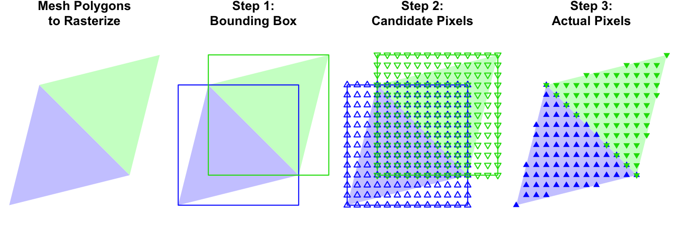
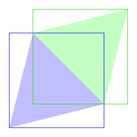
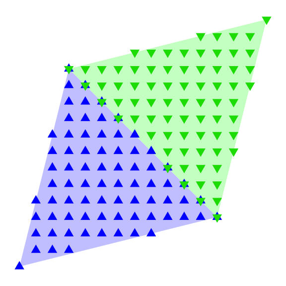
Fortunately for us and our base-R-only challenge, our point cloud is not arbitrary. The source data contains the information required to build the mesh: the original x-y grid. We can generate a tile mesh by subsetting a contiguous portion of our elevation matrix four times, once for each of the four vertices of each tile. This is what it looks like with an illustrative 4 x 4 grid:
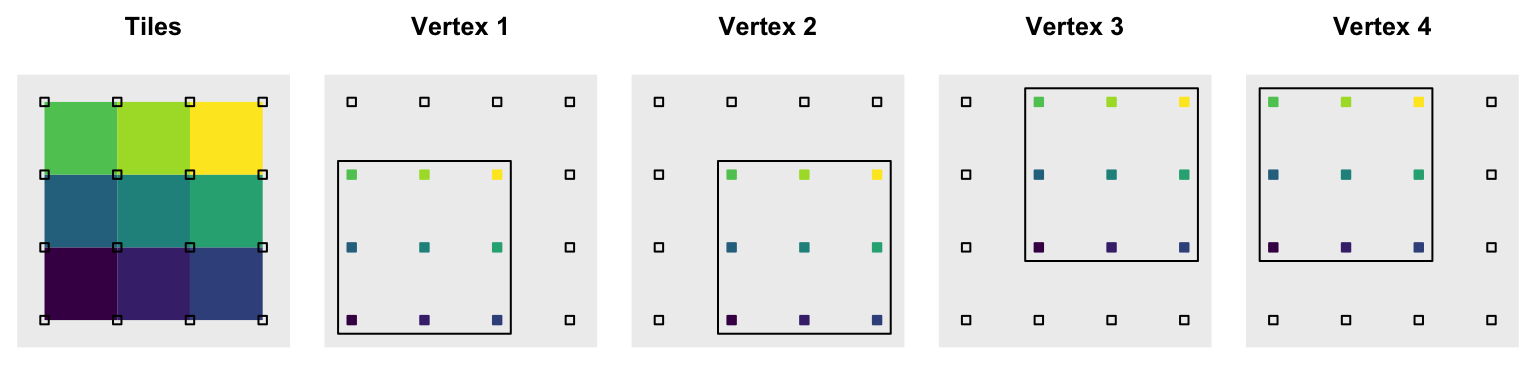
To form each tile as shown in the first panel we take one vertex from each of the four vertex panels. Each panel has the 9 of 16 grid points available for use as vertices enclosed in a black bounding box. For the top left green tile, we take the top left point from each of the bounding boxes. The same process is repeated for each tile by picking the corresponding vertex from each panel. The vertices are colored by the tile they belong to.
The operation we just described is equivalent to alternating dropping the
first/last row/column. Because our projected volcano data is already in long
format, we need to compute which elements in the long data correspond to
the first and last rows. This is actually pretty straightforward if we recall
that our matrix in long format is basically the component vectors “unspooled”.
We can “re-spool” an index vector the length of our data, seq_along(volcano),
by making a matrix out of it with the correct dimensions:
nr <- dim(volcano)[1]
nc <- dim(volcano)[2]
idx.raw <- matrix(seq_along(volcano), nr, nc)
Exploiting the underlying vector nature of matrices, and vice versa, is a common technique when trying to write fast R code.
We can now drop rows and columns in sequence from that index matrix to get the long format indices for each vertex for each tile:
idx.tile <- list(
  v1=c(idx.raw[-nr, -nc]), v2=c(idx.raw[-nr,  -1]),
  v3=c(idx.raw[ -1,  -1]), v4=c(idx.raw[ -1, -nc])
)
For example, to get the location of vertex data for tile forty two:
sapply(idx.tile, '[', 42) v1 v2 v3 v4
42 129 130 43 This means that data for vertex 1 for tile 42 is at position 42 in the long data, for vertex 2 it is at position 129, and so on.
Recall that the volcano data is in vl in long list
format:
str(vl)List of 4
$ x: num [1:5307] -0.4837 -0.0611 0.3615 0.7842 1.2068 ...
$ y: num [1:5307] 35.5 36.6 37.8 39 40.2 ...
$ z: num [1:5307] 93.5 94.1 94.8 95.4 96 ...
$ t: num [1:87, 1:61] 1 1 1 1 1 1 1 1 1 1 ...So to get the x, y, z coordinates, and “texture” values for the vertices
of tile forty two we use:
sapply(vl, '[', sapply(idx.tile, '[', 42)) x y z t
[1,] 16.8 73.1 88.3 1.00
[2,] 15.9 73.8 89.1 0.76
[3,] 16.4 75.0 89.7 0.76
[4,] 17.3 74.3 89.0 1.00In order to extend this to the full tile set we are going to use some for
loops. After all sapply, lapply, and friends are just for
loops themselves. Additionally in this case we want a specific result structure
that is just easier to fill with for loops. Finally, there will only be sixteen
iterations of the loop, so the overhead from R-level function calls is small.
## Initialize result structure
mesh.tile <- matrix(
  list(), nrow=length(idx.tile), ncol=length(vl),
  dimnames=list(names(idx.tile), names(vl))
)
## Fill it with the correctly subset volcano data
for(i in names(idx.tile))
  for(j in names(vl))
    mesh.tile[[i,j]] <- vl[[j]][idx.tile[[i]]]

mesh.tile
x y z t
v1 Numeric,5160 Numeric,5160 Numeric,5160 Numeric,5160
v2 Numeric,5160 Numeric,5160 Numeric,5160 Numeric,5160
v3 Numeric,5160 Numeric,5160 Numeric,5160 Numeric,5160
v4 Numeric,5160 Numeric,5160 Numeric,5160 Numeric,5160This is an instance of the fabled list-matrix. It looks a little weird, but it
is equivalent to a 3D array and is just a list of equal length vectors with a
dim attribute:
length(mesh.tile)[1] 16dim(mesh.tile)[1] 4 4str(mesh.tile[[1]]) num [1:5160] -0.4837 -0.0611 0.3615 0.7842 1.2068 ...One problem with this data structure is that it is duplicative. Most vertices are shared by four tiles, yet we make a copy of each vertex for each tile. This is one of the trade-offs we accept for improved overall performance6.
To extract tile forty two’s data from this structure we can use:
apply(mesh.tile, 1:2, function(x) unlist(x)[42]) x y z t
v1 16.8 73.1 88.3 1.00
v2 15.9 73.8 89.1 0.76
v3 16.4 75.0 89.7 0.76
v4 17.3 74.3 89.0 1.00The required unlist makes this a little awkward, but we do not intend to
operate on a single tile at a time. For most of our manipulations, the
list-matrix is convenient. Look how easy it is to display the mesh from raw
polygons:
zord <- order(Reduce('+', mesh.tile[,'z']))
x <- do.call(rbind, c(mesh.tile[,'x'], list(NA)))[,zord]
y <- do.call(rbind, c(mesh.tile[,'y'], list(NA)))[,zord]
plot_new(x, y)
polygon(rescale(x), rescale(y), col='#DDDDDD', border='#444444')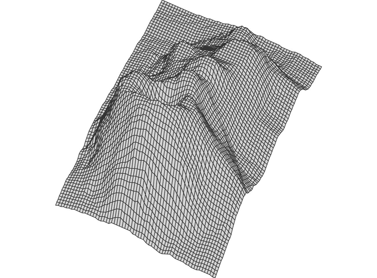
It may help to look at the data structure of x above to understand what’s
going on:
x[,1:10] [,1] [,2] [,3] [,4] [,5] [,6] [,7] [,8] [,9] [,10]
v1 -18.0 -17.1 -16.2 -18.5 -15.3 -17.5 -14.4 -16.6 -18.9 -13.5
v2 -18.9 -18.0 -17.1 -19.4 -16.2 -18.5 -15.3 -17.5 -19.8 -14.4
v3 -18.5 -17.6 -16.7 -18.9 -15.8 -18.0 -14.9 -17.1 -19.4 -14.0
v4 -17.6 -16.7 -15.8 -18.0 -14.9 -17.1 -14.0 -16.2 -18.5 -13.1
NA NA NA NA NA NA NA NA NA NAy shares the same structure. In order to have polygon render multiple
polygons, we need to NA-delimit our input vectors. Rather than painstakingly
creating those vectors from the undelimited ones, we rbind the four vertex
vectors with one NA vector. That this produces a matrix is besides the point;
the idea is that the vector wrapping nature of the matrix allows us to sandwich
NA values between each of our tiles’ data:
c(x[,1:10]) [1] -18.0 -18.9 -18.5 -17.6 NA -17.1 -18.0 -17.6 -16.7 NA -16.2
[12] -17.1 -16.7 -15.8 NA -18.5 -19.4 -18.9 -18.0 NA -15.3 -16.2
[23] -15.8 -14.9 NA -17.5 -18.5 -18.0 -17.1 NA -14.4 -15.3 -14.9
[34] -14.0 NA -16.6 -17.5 -17.1 -16.2 NA -18.9 -19.8 -19.4 -18.5
[45] NA -13.5 -14.4 -14.0 -13.1 NAGreat, but did we really need to subject ourselves to this rigmarole?
Wouldn’t persp, which would still abide by our base-R-only pledge, do this
just as well and without ridiculous list-matrices? Well, kind
of, but more importantly, “this” is not what we’re after.
We have far grander ambitions, and “this” is basically about the limit of what
we can do with persp.
Triangles
A tile mesh is not ideal. Among other things, there is no guarantee the tiles are flat. Triangles on the other hand are guaranteed to be flat, and additionally benefit from simple shading algorithms. So we will turn our tiles into triangles:
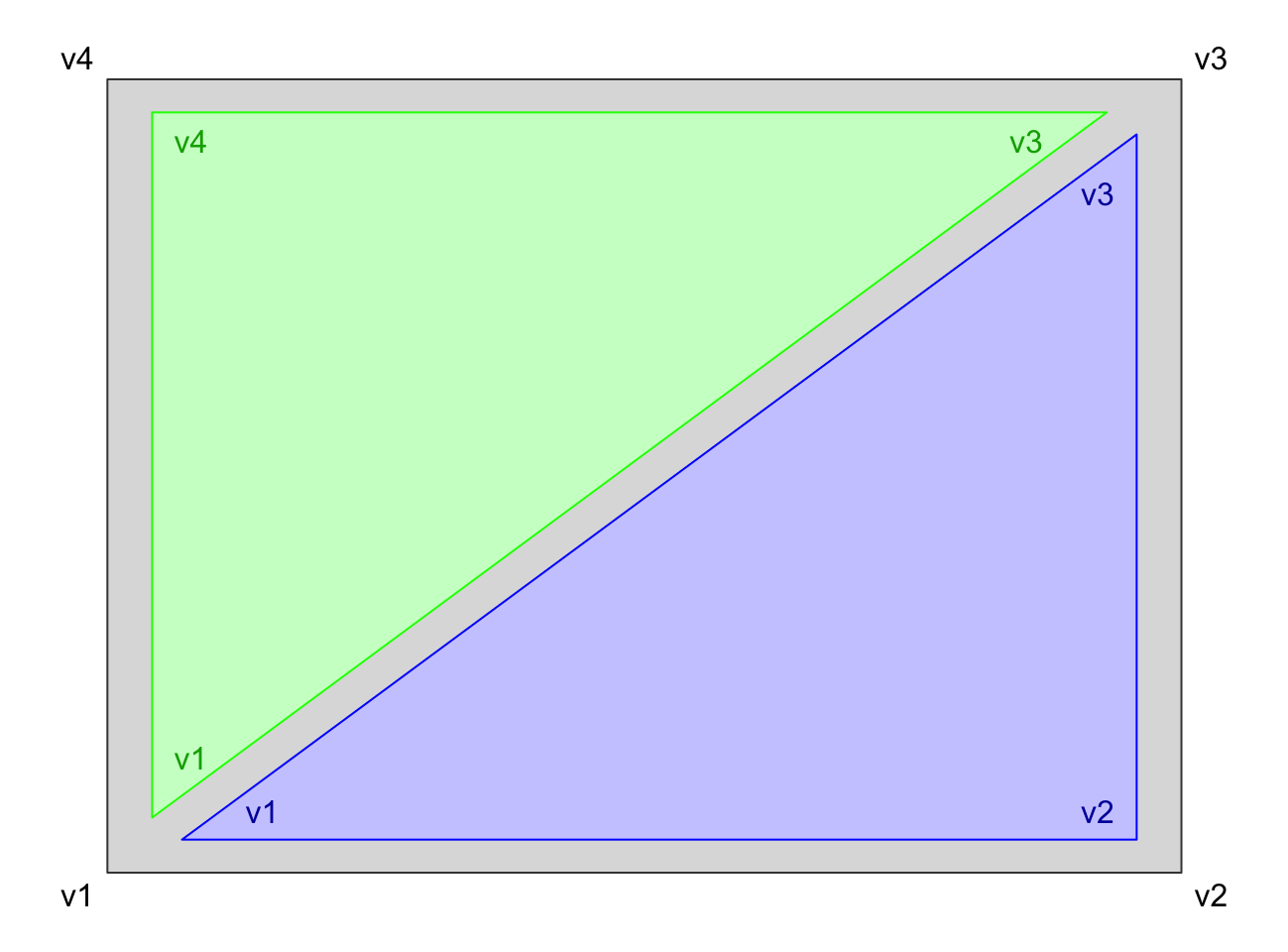
The list-matrix structure of our data makes the translation from tile to triangle mesh trivial:
vertex.blue <- 1:3
vertex.green <- c(3,4,1)
mesh.tri <- Map('c', mesh.tile[vertex.blue,], mesh.tile[vertex.green,])
dim(mesh.tri) <- c(3, 4)
dimnames(mesh.tri) <- list(head(rownames(mesh.tile), -1), colnames(mesh.tile))
mesh.tri
x y z t
v1 Numeric,10320 Numeric,10320 Numeric,10320 Numeric,10320
v2 Numeric,10320 Numeric,10320 Numeric,10320 Numeric,10320
v3 Numeric,10320 Numeric,10320 Numeric,10320 Numeric,10320Plotted:
zord3 <- order(Reduce('+', mesh.tri[,'z']))
x <- do.call(rbind, c(mesh.tri[,'x'], list(NA)))[,zord3]
y <- do.call(rbind, c(mesh.tri[,'y'], list(NA)))[,zord3]
col <- rep(c('#CCCCFF','#CCFFCC'), each=ncol(x)/2)[zord3]
plot_new(x, y)
polygon(rescale(x), rescale(y), col=col)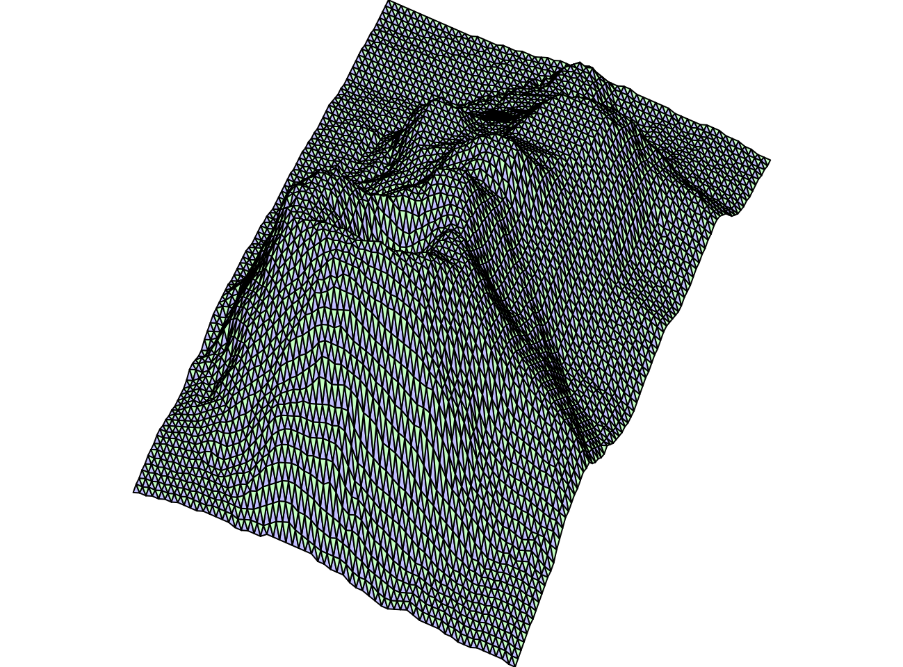
And with more realistic colors by shading each facet with the mean of the vertex shadows:
texture <- gray(Reduce('+', mesh.tri[,'t']) / 3)[zord3]
plot_new(x, y)
polygon(rescale(x), rescale(y), col=texture, border=texture)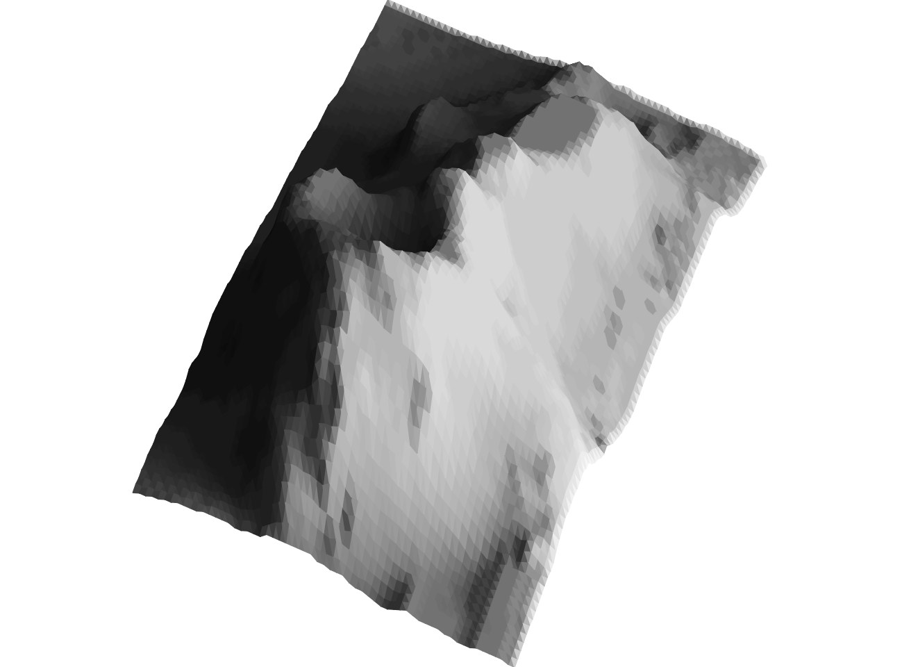
Now we’re cooking!
Perspective
If I had any perspective I wouldn’t be writing this blog post. But that can’t
be helped. Our dear friend volcano is a different story.
Everything we’ve done to this point has assumed no perspective effect; objects of the same size appear the same size irrespective of how far from the observer they are. This observer, you, has been looking at the object along a line parallel to the Z axis and passing through the midpoint of the X and Y extents of the projected object. For expository purposes we are about to, for the first and only time, rotate Observer 0 (you) 90 degrees about the Y axis.
In the following diagram you are looking along a line parallel to the X axis.
The Z axis now runs from left to right. Observers 1, 2, and 3 are all still
looking at volcano along the Z axis:
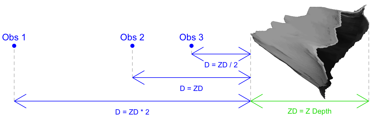
For convenience we define the quantity ZD as the total depth of our object
along the Z axis. Then, we can define the distance of our observers from the
nearest point along the Z axis with the measure D as multiples of ZD.
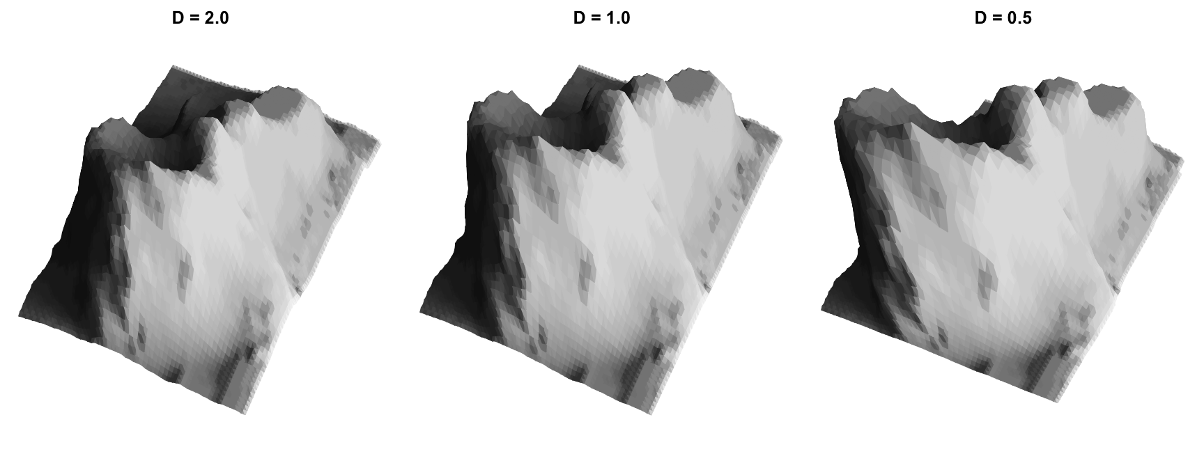
Here is our volcano re-rendered from the perspective of each of observers 1-3 pictured above:
The actual perspective computation is best applied to the original point cloud,
so we go back to the vl variable, which is volcano in
long list format, and apply the perspective transformation
for observer 3:
str(vl) # `volcano` in long list formatList of 4
$ x: num [1:5307] -0.4837 -0.0611 0.3615 0.7842 1.2068 ...
$ y: num [1:5307] 35.5 36.6 37.8 39 40.2 ...
$ z: num [1:5307] 93.5 94.1 94.8 95.4 96 ...
$ t: num [1:87, 1:61] 1 1 1 1 1 1 1 1 1 1 ...D <- 0.5 # Observer 3 is half Z-Depth from volcano
z.rng <- range(vl[['z']])
ZD <- diff(z.rng)
## Center observer on x-y extent and at Z=0
vlp <- vl
vlp[c('x','y')] <- lapply(vl[c('x','y')], function(x) x - sum(range(x)) / 2)
vlp[['z']] <- vlp[['z']] - (z.rng[2] + D * ZD)
## Apply perspective transformation
z.factor <- -1 / vlp[['z']]
vlp[c('x','y')] <- lapply(vlp[c('x','y')], '*', z.factor)Now that we have the perspective-transformed point cloud, we can turn it back
into a triangle mesh. This time we use shadow::mesh_tri, which is a wrapper
around the calculations described in the Mesh section:
mesh.tri <- mesh_tri(vlp, dim(volcano), order=TRUE)
mesh.tri
x y z t
v1 Numeric,10320 Numeric,10320 Numeric,10320 Numeric,10320
v2 Numeric,10320 Numeric,10320 Numeric,10320 Numeric,10320
v3 Numeric,10320 Numeric,10320 Numeric,10320 Numeric,10320x <- do.call(rbind, c(mesh.tri[,'x'], list(NA)))
y <- do.call(rbind, c(mesh.tri[,'y'], list(NA)))
texture <- gray((Reduce('+', mesh.tri[,'t'])/nrow(mesh.tri)))
plot_new(x, y)
polygon(rescale(x), rescale(y), col=texture, border=texture)
mesh_tri has the additional benefit that it orders the tiles by Z value so we
do not need to worry about re-ordering before plotting anymore.
Are we there yet? Nope, we’re going to drag this baby kicking and screaming all the way to its painful, bloody conclusion.
Rasterization
Overview
So far we have relied on base R plotting facilities, polygon mostly, to
actually transform our 3D object representation into an image. There are two
problems with this:
volcanodoes not look very natural with all the triangular faces.- Speed is a problem with higher polygon counts.
We will resolve these issues by resorting to rasterization, whereby we compute what each pixel of our final image should look like. This requires determining which points of our final output pixel grid belong to which triangles. While this is the type of thing a child could do easily, it is surprisingly difficult to instruct a computer to do the same, particularly when we need to account for the need to use internally vectorized7 base R code.
Conceptually, the process takes three steps:
Step 1: Bounding Boxes
 One thing that is easy to do is to compute the rectangular bounding box for each
triangle. All we need to do is compute the x and y extents of the vertices, and
use those to generate the corners of our bounding box.
One thing that is easy to do is to compute the rectangular bounding box for each
triangle. All we need to do is compute the x and y extents of the vertices, and
use those to generate the corners of our bounding box.
Before we do this we need to settle on the resolution of our output grid as everything is going to be measured in relation to that. This is easiest to do with the perspective transformed point cloud data rather than the mesh version. For exposition purposes we keep jumping back and forth between these formats, although in the final rendering pipeline we will only carry out the mesh transformation once we no longer have a need for the point data.
x.width <- 600L
x.rng <- range(vlp[['x']])
y.rng <- range(vlp[['y']])
asp <- diff(y.rng) / diff(x.rng)
y.width <- as.integer(x.width * asp)
vlpt <- vlp
vlpt[['x']] <- rescale(vlpt[['x']], center = 0) * (x.width - 1)  + 1
vlpt[['y']] <- rescale(vlpt[['y']], center = 0) * (y.width - 1) + 1
We can regenerate the mesh, and for each mesh polygon compute the maximum x and y integer pixel values they will contain:
mesh <- mesh_tri(vlpt, dim(volcano), order=TRUE)

ceil_min <- function(x) list(as.integer(ceiling(do.call(pmin, x))))
floor_max <- function(x) list(as.integer(do.call(pmax, x)))

mins <- unlist(apply(mesh[,c('x','y')], 2, ceil_min), recursive=FALSE)
maxs <- unlist(apply(mesh[,c('x','y')], 2, floor_max), recursive=FALSE)
str(mins)  # `maxs` will have same structure
List of 2
$ x: int [1:10320] 272 270 277 275 282 270 280 267 287 275 ...
$ y: int [1:10320] 618 618 616 616 614 613 614 613 612 611 ...We use list(...) in the ceil/floor functions to prevent apply from
simplifying to a numeric matrix, which in turn requires the unlist to get the
desired structure.
This is what bounding boxes look like:
minmax <- unname(c(mins, maxs))
xs <- range(unlist(minmax[c(1,3)]))
ys <- range(unlist(minmax[c(2,4)]))
xss <- lapply(minmax[c(1,3)], function(x) (x - xs[1]) / diff(xs))
yss <- lapply(minmax[c(2,4)], function(y) (y - ys[1]) / diff(ys))
plot_new(xs, ys)
rect(xss[[1]], yss[[1]], xss[[2]], yss[[2]], border='#00000033', asp=1)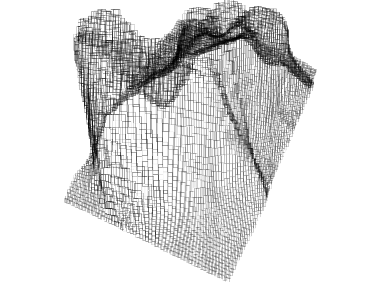
Step 2: Candidate Pixels
We will brute force generate pixels to fill each of our bounding boxes. Oddly this is a little tricky, mostly because we wish to do this fully in internally vectorized code. And it is particularly important that we do so because we are about to dramatically increase the amount of data we are dealing with. The plan of attack is to compute all possible pixel “offset” permutations within each bounding box, and then add back the min x and y coordinates to get the actual pixel coordinates.
First we compute the dimensions of the bounding x/y min/max boxes in pixels:
dims.x <- pmax(maxs[['x']] - mins[['x']] + 1, 0)
dims.y <- pmax(maxs[['y']] - mins[['y']] + 1, 0)
dims.xy <- dims.x * dims.y
Then we generate all the offset permutations. This is the type of thing that
one might normally do with expand.grid:
Map(function(x, y) expand.grid(x=seq_len(x), y=seq_len(y)), dims.x, dims.y)Unfortunately, with 10,320 polygons8 it becomes computationally burdensome.
We can do a little better with lower overhead variations9, but even then we
are left with lists with thousands of elements that are awkward to manage.
Instead we want to generate vectors that contain all the permutations of x and y
offsets we need. We do so here with a toy example for three bounding boxes with
x and y dimensions defined by dim.x0 and dim.y0:
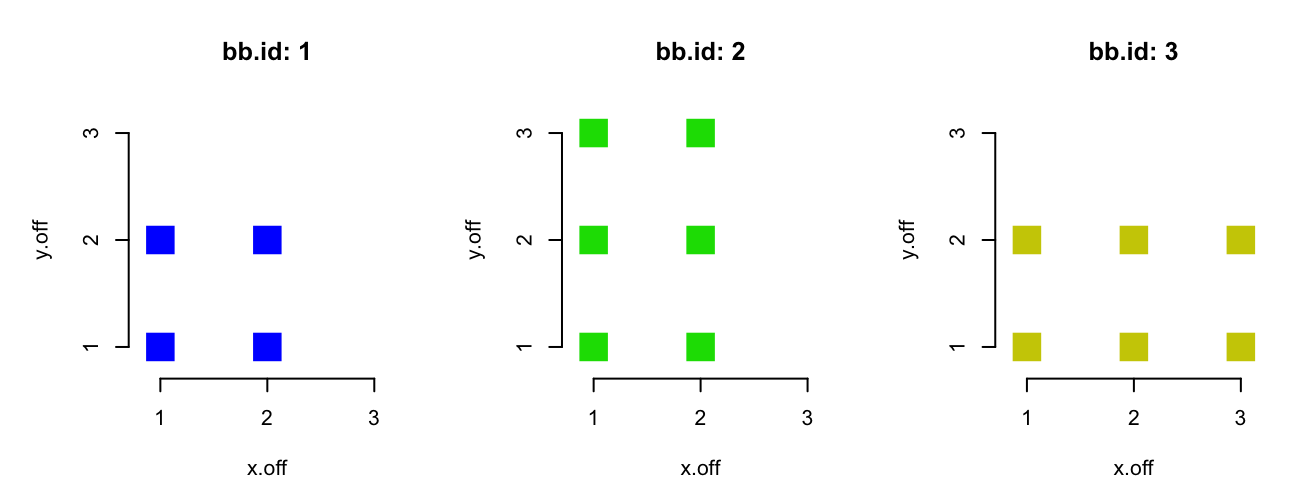
dims.x0 <- c(2, 2, 3)
dims.y0 <- c(2, 3, 2)
dims.xy0 <- dims.x0 * dims.y0

bb.id <- rep(seq_along(dims.xy0), dims.xy0)
Here we took advantage of a less known feature of rep whereby if the second
parameter is the same length as the first, then each value of the first
parameter is repeated the number of times designated by the corresponding value
of the second. Visualized:
bb.id: 1 1 1 1 2 2 2 2 2 2 3 3 3 3 3 3This allows us to generate the bounding box ids with internally vectorized code, despite the bounding boxes having different sizes.
Next we compute the x offsets of each pixel in the bounding box:
## We wish to cycle through the x values in a bounding box
## as many times as there are y values in that bounding box
x.lens <- rep(dims.x0, dims.y0)  # special use of `rep` again here
x.lens
[1] 2 2 2 2 2 3 3## sequence generates sequences of sequences...
x.off <- sequence(x.lens)
x.off [1] 1 2 1 2 1 2 1 2 1 2 1 2 3 1 2 3Now we have all the possible x offset values for each bounding box:
bb.id:  1 1 1 1 2 2 2 2 2 2 3 3 3 3 3 3
x.off:  1 2 1 2 1 2 1 2 1 2 1 2 3 1 2 3
The y offsets are a small variation on the theme:
y.off <- rep(sequence(dims.y0), x.lens)Everything together:
bb.id: 1 1 1 1 2 2 2 2 2 2 3 3 3 3 3 3
x.off: 1 2 1 2 1 2 1 2 1 2 1 2 3 1 2 3
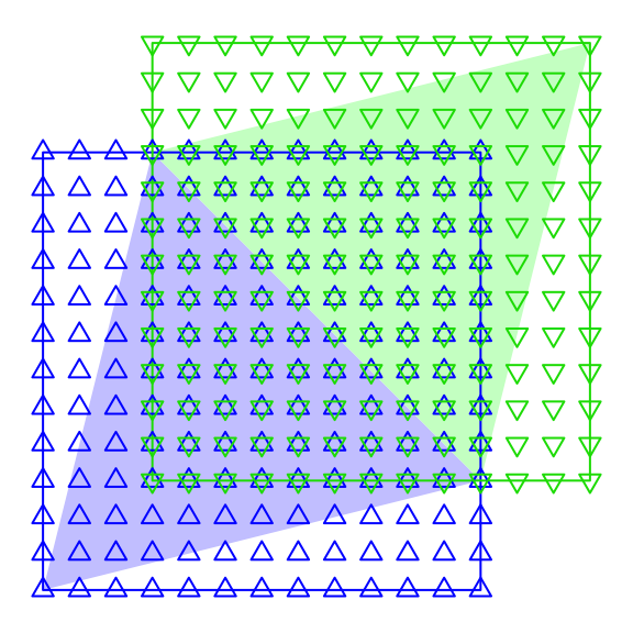
y.off: 1 1 2 2 1 1 2 2 3 3 1 1 1 2 2 2And visualized in two dimensions:
Unfortunately sequence is not an internally vectorized function. It is just a
looped call to seq_len:
sequencefunction (nvec)
unlist(lapply(nvec, seq_len))
<bytecode: 0x7fba7f879790>
<environment: namespace:base>This becomes a liability when we have many sequences as with the full set of
volcano polygons. Fortunately it turns out that it is possible to write an
internally vectorized version of sequence by taking advantage of the
internally vectorized cumulative functions:
## Start with one continuous sequence
x.lens <- rep(dims.x0, dims.y0)
seq <- seq_len(sum(x.lens))

## Compute the locations at which the sequence should reset
reset <- cumsum(x.lens[-length(x.lens)]) + 1L
reset
[1] 3 5 7 9 11 14## Generate a reset vector
sub.raw <- integer(length(seq))
sub.raw[reset] <- reset - 1L
sub.raw [1] 0 0 2 0 4 0 6 0 8 0 10 0 0 13 0 0sub <- cummax(sub.raw)
sub [1] 0 0 2 2 4 4 6 6 8 8 10 10 10 13 13 13## Modify the sequence by subtracting the reset vector
seq - cummax(sub) [1] 1 2 1 2 1 2 1 2 1 2 1 2 3 1 2 3all.equal(x.off, seq - cummax(sub))[1] TRUEThis produces the same result as sequence. For convenience we put the above
logic into shadow::sequence2. Let’s benchmark against the full polygon data:
x.lens <- rep(dims.x, dims.y)   # full volcano bounding boxes
microbenchmark(sequence2(x.lens), sequence(x.lens))
Unit: milliseconds
expr min lq mean median uq max neval
sequence2(x.lens) 13.8 15.9 31.4 22.7 30.8 177 100
sequence(x.lens) 68.8 94.5 139.0 123.2 155.7 363 100We see a 4-5x improvement despite having to rely on far more function calls. Normally we wouldn’t highlight such internal details, but this is an interesting use case of the internally vectorized cumulative functions to solve a problem that doesn’t have a built-in vectorized solution.
Now that we know how we can to generate the candidate x/y offsets quickly we can fill out the bounding boxes.
dims.xy <- dims.x * dims.y
bb.id <- rep(seq_along(dims.x), dims.xy)
x.lens <- rep(dims.x, dims.y)
x.off <- sequence2(x.lens) - 1L
y.off <- rep(sequence(dims.y), x.lens) - 1L

## Add back the min values of the bounding boxes
p.x <- x.off + mins[['x']][bb.id]
p.y <- y.off + mins[['y']][bb.id]
Finally, we’re ready to generate our first pixel-level volcano. We will re-use the textures we computed for our mesh:
p.raster <- matrix(numeric(0), x.width, y.width)
p.raster[cbind(p.x, p.y)] <- rep(texture, dims.xy)
We apply the textures by indexing bb.raster with a matrix (cbind(p.x, p.y)). This is a special type of indexing that allows you to directly address
specific cells by providing a matrix with the row and column values you are
targeting.
There is also a subtle trick deployed here: instead of checking for duplicate pixels we just wrote all the pixels in increasing Z order. This ensures that the pixels nearest to the viewer overwrite those further away implicitly eliminating the duplicates.
Finally, we can plot our matrix as a raster, but due to different conventions about which directions the dimensions run in we need to flip our matrix:
flip <- function(x) t(x)[rev(seq_len(ncol(x))),]
par(mai=numeric(4))
plot(as.raster(flip(p.raster)))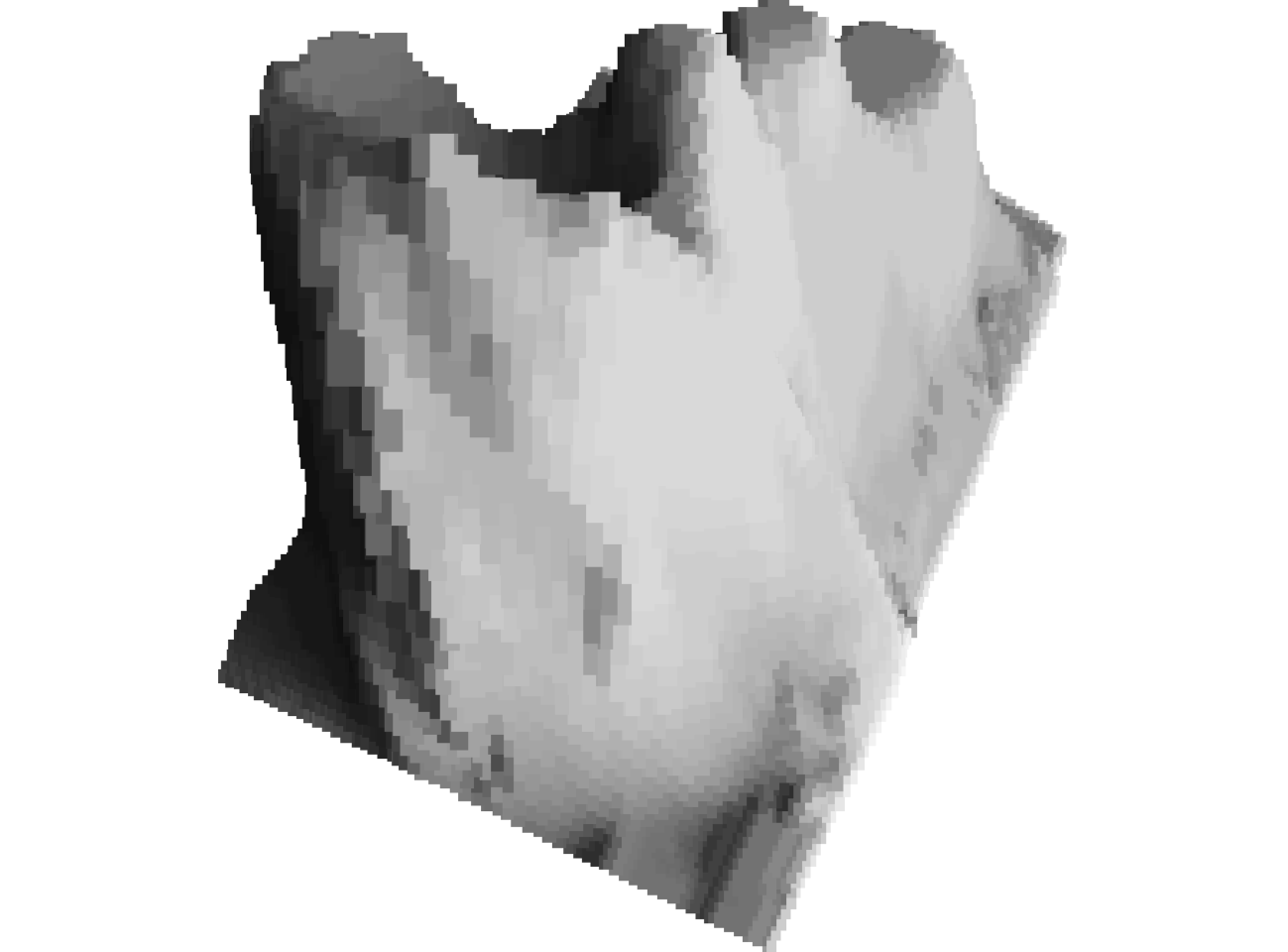
A volcano to make NovaLogic10 proud!
Step 3: Pixel Trimming
 We are now worse off than we were when plotting the polygons in our
mesh, but fear not, we can improve the chunky raster volcano.
We need to trim the excess pixels in our bounding boxes. This is as simple as
deciding which pixels are inside the original polygons and which ones are not.
Really something that a three year old could do. Yet, as is often
the case, expressing such tasks in a way that a computer can easily execute is
difficult.
We are now worse off than we were when plotting the polygons in our
mesh, but fear not, we can improve the chunky raster volcano.
We need to trim the excess pixels in our bounding boxes. This is as simple as
deciding which pixels are inside the original polygons and which ones are not.
Really something that a three year old could do. Yet, as is often
the case, expressing such tasks in a way that a computer can easily execute is
difficult.
There are many possible solutions to the problem, but I settled on using barycentric coordinates. These have the useful property that points with negative barycentric coordinates are outside of the triangle referenced by those coordinates. Additionally, there is a simple arithmetic expression for barycentric coordinates in triangles that can be internally vectorized. Finally, there is a substantial side-benefit that we will discuss when we get to shading.
We are going to re-use the bary_L function we implemented as part of our
previous blog post on list data structures and vertex shading. See that
blog post for a detailed explanation of what the function does. For now, all we
care about is which points end up with negative barycentric coordinates.
shadow::barycentric is a copy of that function.
First we need to match up our vertex data to the candidate points so we can use vectorized operations. Unfortunately, this means that we have to make a copy of the vertex x-y coordinates for every single point. This is wasteful, but one of the trade offs often made in R: use more memory in order to make fewer expensive R function calls.
cols <- c('x','y','t')  # don't need Z vals as `bb.id` already Z ordered
mesh.all <- mesh[, cols]
mesh.all
x y t
v1 Numeric,10320 Numeric,10320 Numeric,10320
v2 Numeric,10320 Numeric,10320 Numeric,10320
v3 Numeric,10320 Numeric,10320 Numeric,10320## each id in `bb.id` reference a mesh triangle
mesh.all[] <- lapply(mesh.all, '[', bb.id)
mesh.all x y t
v1 Numeric,1302788 Numeric,1302788 Numeric,1302788
v2 Numeric,1302788 Numeric,1302788 Numeric,1302788
v3 Numeric,1302788 Numeric,1302788 Numeric,1302788Now we have as many polygons as points, which allows us to compute the barycentric coordinates in one R function call:
bc <- barycentric(list(x=p.x, y=p.y), mesh.all[,c('x','y')])
str(bc)
List of 3
$ : num [1:1302788] 0.4138 0.2552 0.0966 -0.062 -0.2205 ...
$ : num [1:1302788] -0.436 -0.203 0.029 0.261 0.494 ...
$ : num [1:1302788] 1.022 0.948 0.874 0.801 0.727 ...Of the five points str shows, only point 3 will be kept as it is the only one
with positive barycentric coordinates for each vertex.
## determine which points are inbounds and generate raster matrix
inbounds <- Reduce('&', lapply(bc, '>=', 0))

p.x.in <- p.x[inbounds]
p.y.in <- p.y[inbounds]
p.raster <- matrix(numeric(0), x.width, y.width)
p.raster[cbind(p.x.in, p.y.in)] <- rep(texture, dims.xy)[inbounds]

par(mai=numeric(4))
plot(as.raster(flip(p.raster)), asp=1)![]()
Great! All that work and we’re right back were we started11 with our triangle mesh. But isn’t it so satisfying that we built this thing pixel by pixel, with our bare hands. It’s a little bit like that pasta sauce you might make from scratch, that objectively really isn’t that much better than the stuff in the jar, but it sure does seem to taste better.
Oh, and we’re not done yet.
Shading
The main reason I picked barycentric coordinates to determine which points are inbounds is that those coordinates also represent the relative weights at each vertex of the triangle required to “balance” the triangle on the corresponding points. This will allow us to shade the pixels within polygons based on their proximity to each vertex and the vertex colors. I cover this at length in the previously mentioned blogpost.
Since we have the barycentric coordinates, all we have to do is compute weighted average colors for each pixel:
bc.in <- lapply(bc, '[', inbounds)
t.in <- lapply(mesh.all[, 't'], '[', inbounds)
t.shaded <- Reduce('+', Map('*', t.in, bc.in))

p.raster <- matrix(numeric(0), x.width, y.width)
p.raster[cbind(p.x.in, p.y.in)] <- t.shaded

par(mai=numeric(4))
plot(as.raster(flip(p.raster)))
And just like that we have a beautifully shaded volcano!
Interlude II
Hah, you probably thought we were done. Well, we’re close. But first,
we need to run some benchmarks. I captured the entire process we went through
in shadow::render to make it easier to re-use and benchmark:
treeprof::treeprof(
  render_elevation(volcano, shadow, rot, resolution=600, d=.5)
)
Ticks: 3743; Iterations: 10; Time Per: 520.3 milliseconds; Time Total: 5.203 seconds; Time Ticks: 3.743
milliseconds
render_elevation --------------------- : 520.3 - 0.0
rasterize ------------------------ : 518.2 - 8.9
barycentric ------------------ : 132.8 - 132.8
mesh_expand ------------------ : 120.7 - 0.0
| lapply ------------------- : 120.7 - 120.7
candidate_pixels ------------- : 102.7 - 69.5
| sequence2 ---------------- : 33.2 - 12.1
| cummax --------------- : 16.0 - 16.0
| integer -------------- : 4.9 - 4.9
lapply ----------------------- : 55.9 - 55.9
shade ------------------------ : 48.7 - 0.0
| Reduce ------------------- : 48.7 - 0.0
| Map ------------------ : 42.7 - 0.0
| | mapply ----------- : 42.7 - 0.0
| | lapply ------- : 34.1 - 34.1
| | <Anonymous> -- : 8.6 - 8.6
| f -------------------- : 6.0 - 6.0
Reduce ----------------------- : 45.0 - 0.7
f ------------------------ : 23.1 - 23.1
lapply ------------------- : 21.3 - 0.0
FUN ------------------ : 21.1 - 21.1Almost 2FPS! We’re not going to be playing any 3D games with this, but considering this is done on a 2016 Macbook (yes, the 12" Macbook a.k.a. Apple Netbook), on CPU, with a single core, in double precision floating point12, and via an interpreted programming language, it’s not too bad.
As for the benchmark details: virtually all the time was spent rasterizing. 3D
projection, meshes, and perspective adjustments take no time, relatively
speaking. So why bother with rasterization? One obvious answer is that it
allows us to implement much better shading. We also want the bitmap data
as an R object for further manipulation, and while it is possible to save
the polygon output to image files, I don’t know of an easy way to get that
information back into R with base-R-only. And finally polygon rendering becomes
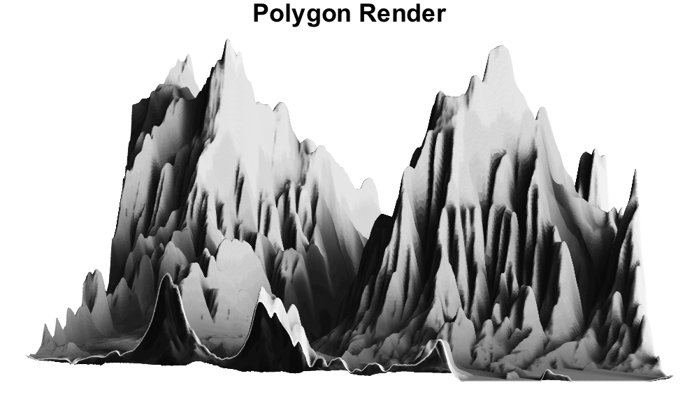
expensive when the polygon counts increase. Here we illustrate with an
elevation map that has fifty times as many points as volcano:
# File originally from http://tylermw.com/data/dem_01.tif.zip
elev2 <- readRDS('static/data/three-d-pipeline-elev-complex.RDS')
# shadow2 <- ray_shade2(elev2, seq(-90, 90, length=25), 45)
shadow2 <- readRDS('static/data/three-d-pipeline-shadow-complex.RDS')
rot2 <- rot_x(-90) %*% rot_z(-90)

system.time({
  rel <- render_elevation(elev2, shadow2, rot2, 1000, 2, zord='pixel', empty=1)
  par(mar=c(1,0,1,0))
  plot(as.raster(flip(rel)))
  title('Raster Render', cex=1.5)
})
user system elapsed
1.956 0.649 2.622system.time({
mesh2 <- elevation_as_mesh(elev2, shadow2, rot_x(-90) %*% rot_z(-90), d=2)
x <- do.call(rbind, c(mesh2[,'x'], list(NA)))
y <- do.call(rbind, c(mesh2[,'y'], list(NA)))
texture <- gray((Reduce('+', mesh2[,'t'])/nrow(mesh2)))
par(mar=c(1,0,1,0))
plot.new()
polygon(rescale(x), rescale(y), col=texture, border=texture)
title('Polygon Render', cex=5)
}) user system elapsed
10.389 0.238 10.664It is unclear to me why the polygon method is slower13 given that the graphical device will rasterize the polygons as well, presumably in compiled code. With the higher polygon count, the polygon image quality is higher, but if you compare the two renders closely you look closely you can still see the polygon artifacts:
![]()
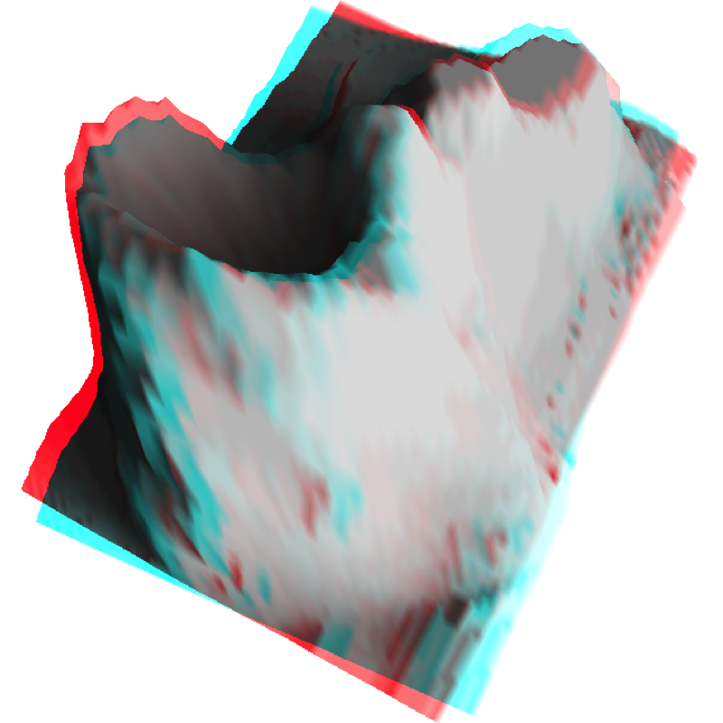
Stereoscopy
Finally: the fun stuff. As hinted at in the introduction, we are looking to
make analygraphs and stereograms. We can easily render two scenes
with slightly different angles. For convenience, we use
shadow::mrender_elevation which is a wrapper to render_elevation for
multiple rotations. In addition to supporting multiple rotations,
mrender_elevation uses absolute distances and fixed fields of view to ensure
consistent perspective transformations.
rot.l <- rot %*% rot_z(2.5)
rot.r <- rot %*% rot_z(-2.5)
elren <- mrender_elevation(
  volcano, shadow, list(rot.l, rot.r), res=1000, d=125, fov=85
)
left <- flip(elren[[1]])
right <- flip(elren[[2]])
In order to generate an analygraph we need to assign the left image to the red channel, and the right image to the cyan channel. No cyan channel? No problem: turns out that cyan is just blue and green added together. This is very easy to do as the R raster format accepts 3D arrays as inputs, where each value of the third dimension corresponds to one of the RGB color channels:
analygraph <- function(left, right) {
  analygraph <- array(0, dim=c(dim(left), 3))
  analygraph[,,1] <- left      # red channel
  analygraph[,,2:3] <- right   # green and blue
  analygraph
}
elcolor <- analygraph(left, right)
par(bg='black', mai=numeric(4))
plot(as.raster(elcolor))
shadow::analygraph_glasses(.15)   # for the icon h/t @jurbane2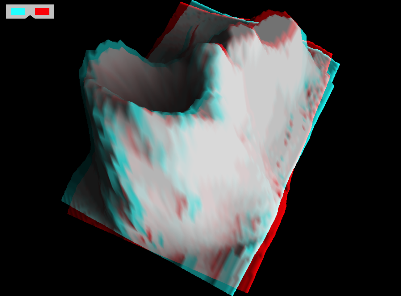
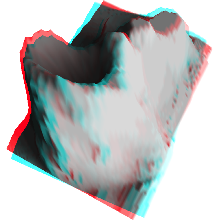
You can get analygraph glasses very cheaply. I got ten for five bucks.
One advantage of using red and cyan is that the areas where the images overlap are white or gray, which looks a lot more natural. If we had used red and green the overlapping areas would end up yellow.
If you can’t be bothered getting the glasses, we can also make stereograms:
eljuxt <- cbind(left, right)
par(bg='black', mai=c(.25, .5, .25, .5))
plot(as.raster(eljuxt))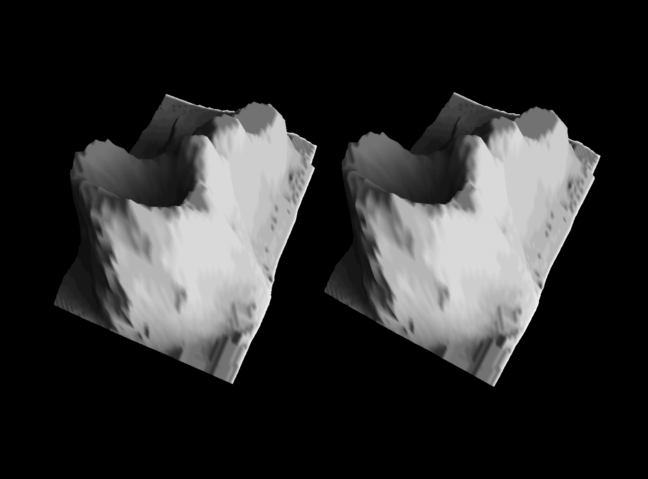
In order to see the 3D effect on these you need to get your eyes to diverge such that each eye is looking at one of the images. It does take practice to master. One trick that can help is making the image smaller so that the volcanoes are closer together. If you wear glasses you might also find it easier to “focus” on the stereogram with them off. The effort is worth it as the perspective effect is much stronger with stereograms than with analygraphs.
Since nowadays it seems no blog post is complete without some kind of animation,
let’s spin up volcano. Out of courtesy to those of you who get nauseated
easily, I’m not auto-playing the videos. I also set up the lighting to remain
constant throughout so that it is clear that our frame of reference is fixed.
Tough luck to those visiting volcano today.
And one more, why not?
Assembling the video from the component frames with ffmpeg magic
and using blogdown to render the post are the only things we resorted to
non base R for.
So Long, and Thanks For All The Clicks
Hopefully this was somewhat instructive and enjoyable for you. I imagine if you got this far there is a chance it was. Or maybe you’re just looking for my contact info to flame me on the interwebs. If the latter I’ll take some solace in the fact that you probably overshot and had to scroll back through the footnotes and appendix.
All the illustrations in this post were generated with base R graphics. You can see the source for this post on Github.
Appendix
Session Info
sessionInfo()R version 3.6.2 (2019-12-12)
Platform: x86_64-apple-darwin15.6.0 (64-bit)
Running under: macOS Mojave 10.14.6
Matrix products: default
BLAS: /Library/Frameworks/R.framework/Versions/3.6/Resources/lib/libRblas.0.dylib
LAPACK: /Library/Frameworks/R.framework/Versions/3.6/Resources/lib/libRlapack.dylib
locale:
[1] en_US.UTF-8/en_US.UTF-8/en_US.UTF-8/C/en_US.UTF-8/en_US.UTF-8
attached base packages:
[1] stats graphics grDevices utils datasets methods base
other attached packages:
[1] shadow_0.0.0.9000
loaded via a namespace (and not attached):
[1] compiler_3.6.2 magrittr_1.5 bookdown_0.10 tools_3.6.2
[5] htmltools_0.3.6 yaml_2.2.0 Rcpp_1.0.1 fansi_0.4.1
[9] stringi_1.4.3 rmarkdown_1.12 blogdown_0.12 knitr_1.23
[13] stringr_1.4.0 digest_0.6.20 xfun_0.8 evaluate_0.14 Helper Functions
## Rescale data to a range from 0 to `range` where `range` in (0,1]
rescale <- function(x, range=1, center=0.5)
  ((x - min(x, na.rm=TRUE)) / diff(range(x, na.rm=TRUE))) * range +
   (1 - range) * center

## Prepare a plot with a particular aspect ratio
plot_new <- function(
  x, y, xlim=c(0,1), ylim=c(0,1),
  par.args=list(mai=numeric(4L), xaxt='n', yaxt='n', xaxs='i', yaxs='i')
) {
  if(length(par.args)) do.call(par, par.args)
  plot.new()
  plot.window(
    xlim, ylim, asp=diff(range(y, na.rm=TRUE))/diff(range(x, na.rm=TRUE))
) }
Meshes With Persp
With some work I was able to roughly recreate our own tile mesh:
par(mai=numeric(4))
persp(
  x=seq_len(nrow(volcano)), y=seq_len(ncol(volcano)), z=volcano,
  ylim=c(2,52), xlim=c(6,46), theta=-65, phi=70,
  col='#DDDDDD', border='#444444', r=1e7, scale=FALSE
)
Warning in persp.default(x = seq_len(nrow(volcano)), y =
seq_len(ncol(volcano)), : surface extends beyond the box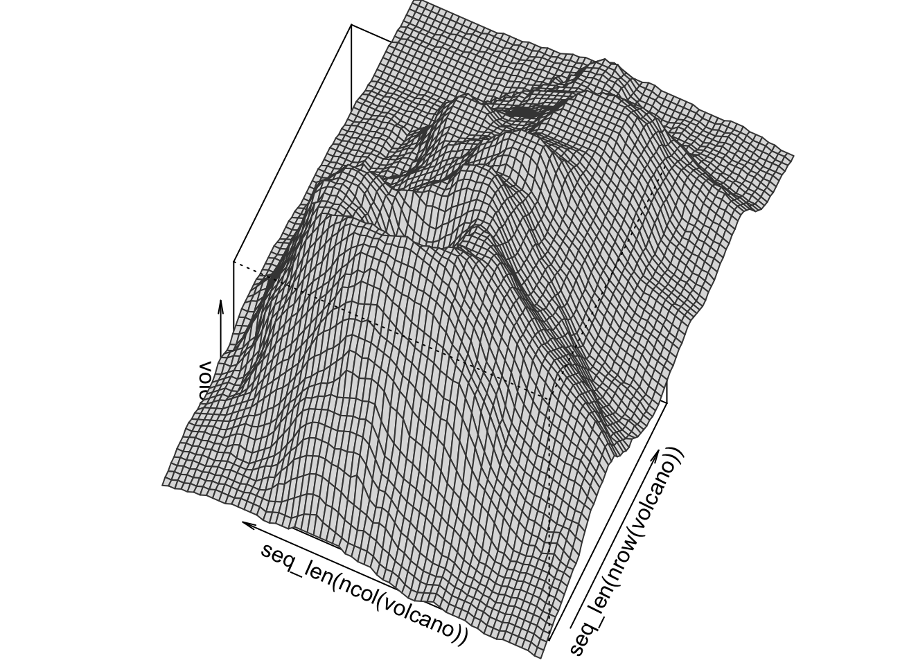
I left the box in on purpose to highlight that I had to go to ridiculous lengths
to get persp to fit the viewport the way I wanted. Finding the correct xlim
and ylim values to achieve the desired effect was an exercise in almost futile
stochastic debugging. There probably is a way to do this better.
Notice also that the theta and phi values are kind of weird given that we
use rot_x(-20) %*% rot_z(65). I wasn’t able to figure out what values I
needed until I went through the C source code to figure out what what order
phi and theta were being applied (it matters), and saw this:
## r-devel@75683:src/library/graphics/src/plot3d.c@1205
XRotate(-90.0);                /* rotate x-y plane to horizontal */
YRotate(-theta);               /* azimuthal rotation */
XRotate(phi);                  /* elevation rotation */
I had similar frustrations in understanding rgl as well, and similarly had to
dig through sources to figure exactly what was going on and eventually decided
it was more fun to just build the whole thing from scratch to best fit the
specific purpose I had in mind.
As far as I was able to get with persp is this:
par(mai=numeric(4))
tile.col <- Reduce('+', mesh.tile[,'t']) / 4
persp(
  x=seq_len(nrow(volcano)), y=seq_len(ncol(volcano)), z=volcano,
  ylim=c(2,52), xlim=c(6,46), theta=-65, phi=70,
  col=gray(tile.col), border=NA, r=1e7, scale=FALSE, box=FALSE
)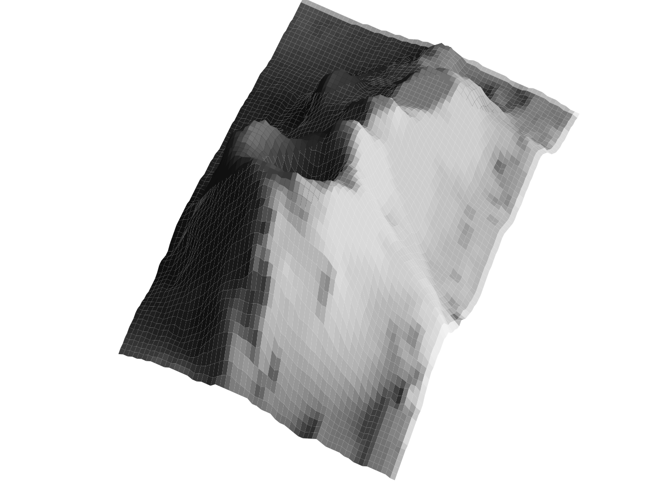
This doesn’t look great: it’s blocky, and there is no good way to
get rid of the anti-aliasing lines. I also used our mesh.tile
list-matrix to compute the shading of the tiles, which requires a fair bit of
work beyond what persp does on its own. Finally, while I can get this
out to a bitmap, AFAICT there is no easy base-R-only way to read back a bitmap
into R for manipulation to make the analygraphs.
Videos
Both videos were made by generating PNG files that I turned into an MP4 with ffmpeg` with the command:
ffmpeg -pattern_type glob -i '*.png' -r 30 -pix_fmt yuv420p out.mpAnalygraph videos:
## Basic video
deg <- 0:119 * 3
deg.stereo <- c(deg + 2.5, deg - 2.5)
rot.360 <- lapply(deg.stereo, function(x) rot %*% rot_z(x))
sun.els <- seq(-30, 120, length=50)
shadows <-
lapply(deg + 180, ray_shade2, anglebreaks=sun.els, heightmap=volcano)
elren <- mrender_elevation(volcano, shadows, rot.360, res=600, d=200)
elren <- lapply(elren, flip)
dim(elren) <- c(length(elren) / 2, 2) # a list matrix again
elrows <- seq_len(nrow(elren))
elren2 <- lapply(elrows, function(i) do.call(analygraph, elren[i,]))
size <- max(dim(elren2[[1]]))
for(i in elrows) {
png(sprintf('tmp/volc%03d.png', i), width=size, height=size, bg='black')
par(mai=numeric(4))
plot(as.raster(elren2[[i]]))
analygraph_glasses(.15)
dev.off()
}
## Coming at ya video
eye.sep <- tan(2.5/180*pi) * 200 # really half eye sep, exaggerate angle
dists <- seq(1400, 50, length.out=90)
deg.d <- atan(eye.sep / dists) * 180 / pi
deg.ds <- c(deg.d, -deg.d)
rot.d <- lapply(deg.ds, function(x) rot %*% rot_z(x))
elrena <- mrender_elevation(volcano, shadow, rot.d, res=600, d=as.list(dists))
elrena <- lapply(elrena, flip)
dim(elrena) <- c(length(elrena) / 2, 2) # a list matrix again
elrows <- seq_len(nrow(elrena))
elrena2 <- lapply(elrows, function(i) do.call(analygraph, elrena[i,]))
size <- max(dim(elrena2[[1]]))
for(i in elrows) {
png(sprintf('tmp1/volc%03d.png', i), width=size, height=size, bg='black')
par(mai=numeric(4))
plot(as.raster(elrena2[[i]]))
analygraph_glasses(.15)
dev.off()
}Stereogram video:
elren3 <- lapply(elrows, function(i) do.call(cbind, elren[i,]))
width <- ncol(elren3[[1]]) / 2
height <- nrow(elren3[[1]]) / 2
for(i in elrows) {
  path <- sprintf('tmp2/volc%03d.png', i)
  png(path, width=600, height=600/width*height, bg='black')
  par(mai=numeric(4))
  plot(as.raster(elren3[[i]]))
  dev.off()
}
Why would I subject myself to this? Well, I’m a sucker for learning new interesting things such as how 3D rendering is actually done, and there is no better way to learn than to do. I also believe, as an R package developer, that it is important to know just how far you can push base R (there are good reasons for this that I will elaborate on in a future blog post), and there is no better way to know than to push it to do things it isn’t really meant to do.↩
We’re not shooting for live rendering of 3D games here; something that will allow us to render short video clips in single digit minutes is what we consider useful.↩
I use the term loosely to mean the packages that are by default loaded into the search path of a “vanilla” R session. As of this writing the packages are
stats,graphics,grDevices,utils,datasets,methods, and the actualbasepackage.↩Some 3D packages out there will blatantly lie to you by rotating the displayed axes along with the object, making it seem like the axes are rotating, but in reality the underlying axes are not rotating. This lie made it particularly difficult for me to figure out why things were not rotating the way I thought they should. I’m still pissed off about it.↩
We’re not shooting for live rendering of 3D games here; something that will allow us to render short video clips in single digit minutes is what we consider useful.↩
There is always a tension in R between minimizing R-level function calls and minimizing memory footprint. Due to the cost of calling R-level functions it is often though not always useful to duplicate or partially duplicate data if it avoids many R-level function calls.↩
R code that carries out looped operations over vectors in compiled code rather than in R-level code.↩
In reality we only need to do this for the polygons that are visible in the end result, but determining what is visible and not is non-trivial, particularly for open surfaces at the pixel level, so we’ll reserve that for a possible future low-probability-of-getting-made blog post.↩
A more efficient variation on
expand.grid(x, y)would belist(rep(seq_len(x),y), rep(seq_len(y), each=x))↩NovaLogic developed a 3D terrain rendering engine for use in the Comanche helicopter flight simulations back in the early nineties. It was awesome then, but looks about as good as our volcano here does right now:

See s-macke for an amazing explanation of their rendering engine.↩Well, almost, the eagle-eyed reader will notice we’ve lost the anti-aliasing, but shhhh, don’t tell anyone.↩
3D rendering is typically done in single precision floating point, which would halve the memory footprint of the process. Granted we only have on color chanel, but on the whole even if we had three color chanels we’re taking a performance penalty due to R only have one type of floating point data type.↩
Possibly it is because the device still renders the polygon borders, or perhaps because of anti-aliasing (though turning that off did not seem to make a difference). I am not curious enough to look at the source of the device code.↩