I Got Sucked In

Over the past few months I’ve resisted distraction by the pretty awesome work that Tyler Morgan Wall has been doing with his rayshader package. His blog post on the topic is visually stunning, accessible, and pedagogically effective. So I admired the lively reliefs that cropped up on twitter and left it at that.

But then others picked on the rayshading algorithm to make a point about the incorrigible slowness of R, and the combination of cool graphics and an insult on R’s good name is simply too much for me to ignore.

R is not that slow! Figure 1 below was rendered with a pure-R ray-shader:

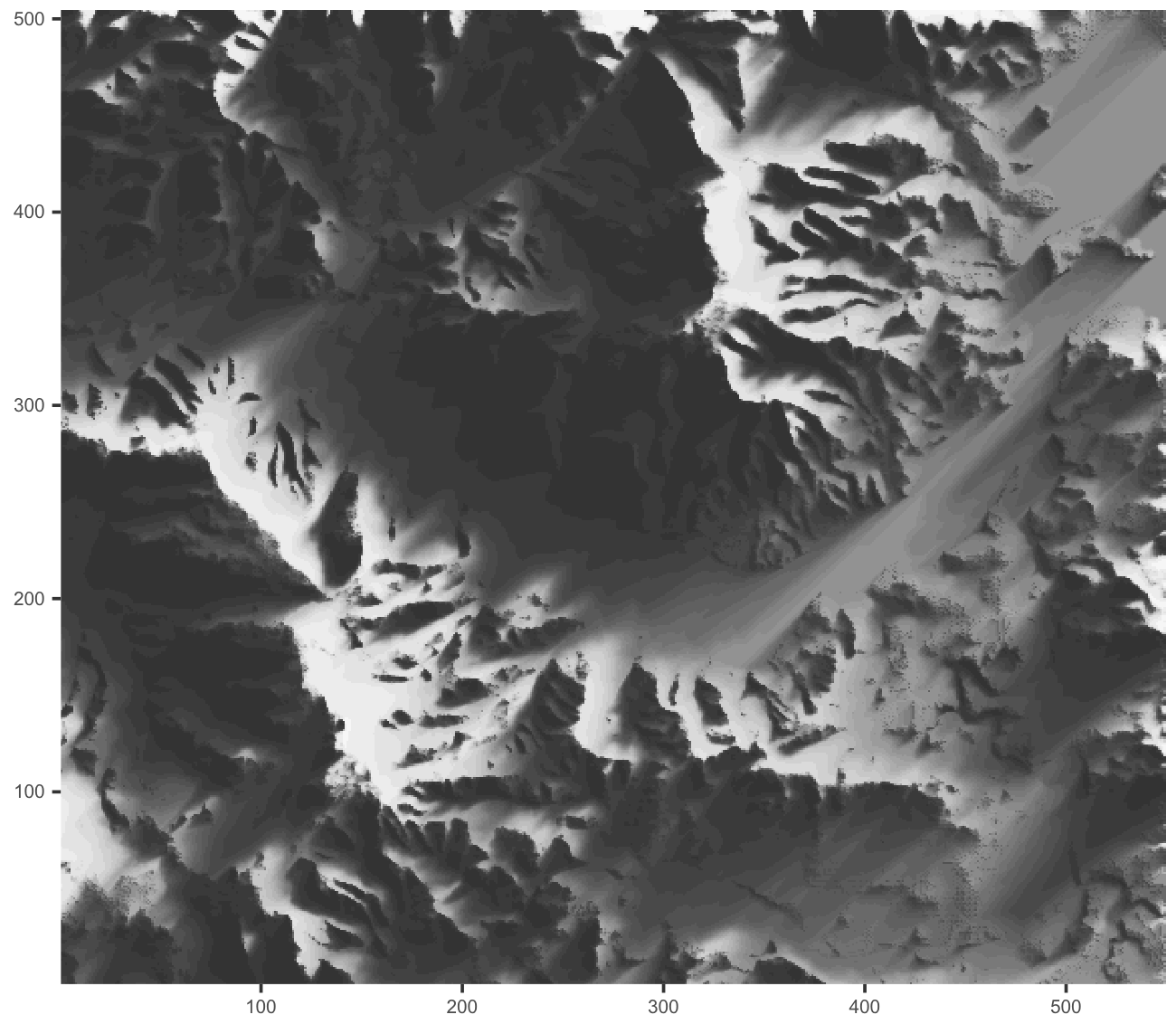
Fig. 1: Shaded mountains - vectorized R rendering

It took ~15 seconds on my system. rayshader::ray_shade, which is written in C++, takes over 20 seconds to do the same.

This post is not about whether rayshader should be written in pure R (it should not be); it is just a case study on how to write reasonably fast pure-R code to solve a problem that on its face does not seem well suited to R.

R Can be Slow

The benchmarks that sucked me into this are from Wolf Vollprecht’s Next Journal article (Fig 2):

Fig. 2: Vollprecht Benchmarks

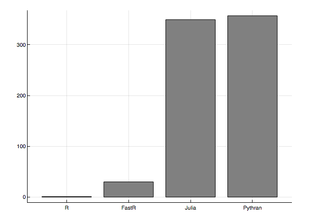
The height of the bars represent the speed-up factor relative to the simple R implementation.

R function calls are expensive, so any time you have nested R loops calling lots of R functions, you will have a slow program, typically two orders of magnitude slower than compiled code. This lines up with what the benchmarks above, and is not surprising if you consider that the original R implementation has a quadruple nested loop in it:

for (i in 1:nrow(heightmap)) {      # for every x-coord
  for (j in 1:ncol(heightmap)) {    # for every y-coord
    for (elevation in elevations) { # for every sun elevation
      for (k in 1:maxdistance) {    # for each step in the path
        # does ray hit obstacle?
} } } }

heightmap is an elevation matrix. In figure one it is 550 x 505 pixels, so with 25 elevations and 100 step paths this requires up to 700 million calls of the innermost routine. The most trivial R primitive function evaluations take ~100ns and closer to ~500ns for non-primitive ones. The math is harsh: we’re looking at up to 70 - 350 seconds per operation used by our ray shading algorithm.

If R is Slow For You, You’re Probably Doing it Wrong

Sure, you can use quadruple nested loops in R, but those are really meant for the ice rink, not R. There are hundreds of R functions and operators that implicitly loop through vector objects without invoking an R function for each element. You can write fast R code most of the time if you take advantage of those functions.

We turned the original for loop R code into a function, and wrote an internally vectorized version of it without for loops. These are called ray_shade1 (for loop) and ray_shade2 (vectorized) respectively, and are part of the shadow demo package.

We timed the for loop, vectorized, rayshader::rayshade C++, and even the Julia version from the Wolf Vollprecht’s Next Journal article, but this time we used the more substantial data set from figure 1:

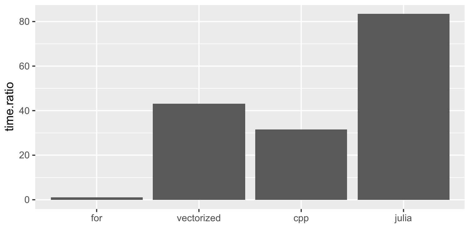
The vectorized R version is 40-50x faster than the original for loop version. The Julia version is another ~2x faster. I did observe a 160x speedup for the smaller volcano elevation map with Julia, but it seems Julia’s advantage is not as marked with a more realistic file size. I did notice that Julia’s benchmarks are using a 32bit float instead of the 64bit ones used by R, but changing that only has a moderate (~15%) effect on performance.

One surprising element in all this is how slow the C++ version from the rayshader package runs. I would have expected to run neck and neck with the Julia version. Turns out that this slowness is caused by checking for user interrupts too frequently. I imagine that the next version (>0.5.1) of rayshader::ray_shade will be closer to the Julia one.

Compiled code will almost always be faster than pure R code, but in many cases you can get close enough in pure R that it is not worth the hassle to switch to compiled code, or to a language that is not as stable and well supported as R.

And to confirm we are actually doing the same thing:

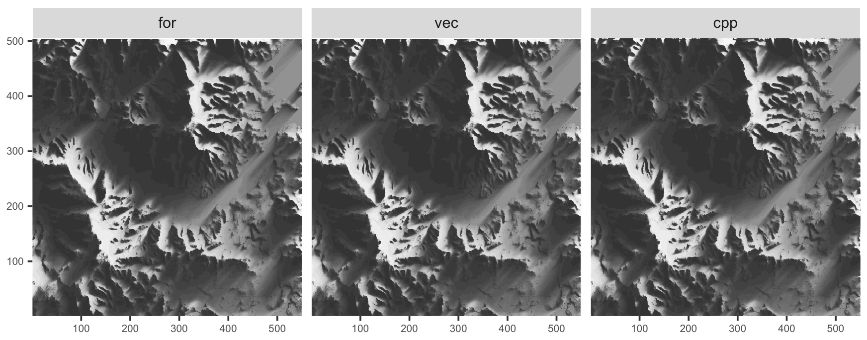
Fig. 4: Mountain landscape shaded with three methods.

We are not showing the Julia output, but we confirmed visually that it looks the same. The various R versions shown here are not exactly identical, partly due to numeric precision issues, partly because the original R algorithm and the C++ treat the boundary of the plot differently.

How Do We Write Fast R Code?

Minimize R-Level Loops

As a rule of thumb: if you have an algorithm that iterates over items, and the result of computing each item is independent of the others, you should be able to write a reasonably fast R solution so long as you do not rely on R-level loops. R-level loops include explicit for loops, but also loops carried out via the *ply family of functions. In some cases it is okay to use R-level loops for the outer loop, so long as the inner loops call internally vectorized code.

Here is an example where we use an explicit R loop to compute a sum of a vector, vs an internally C-vectorized version of the same thing:

v <- runif(1e4)
sum_loop <- function(x) {
  x.sum <- 0
  for(i in x) x.sum <- x.sum + i
  x.sum
}
v.sum.1 <- 0
microbenchmark::microbenchmark(times=10,
  v.sum.1 <- sum_loop(v),
  v.sum.2 <- sum(v)
)

Unit: microseconds
                   expr   min    lq   mean median    uq   max neval
 v.sum.1 <- sum_loop(v) 439.7 455.4 4456.0  485.1 512.4 40177    10
      v.sum.2 <- sum(v)  20.2  21.1   48.5   23.5  27.9   270    10

v.sum.1 == v.sum.2

[1] TRUE

The one-to-two orders of magnitude difference in timing is typical.

To internally vectorize ray_shade2 we had to:

Change the inner function to vectorize internally.
Manipulate the data so that the interpolation function can operate on it once.

Part 1: Internally Vectorize Inner Function

In our case the key inner function is the bilinear interpolation used to interpolate relief height along our “shade-rays”:

faster_bilinear <- function (Z, x0, y0){
  i = floor(x0)
  j = floor(y0)
  XT = (x0 - i)
  YT = (y0 - j)
  result = (1 - YT) * (1 - XT) * Z[i, j]
  nx = nrow(Z)
  ny = ncol(Z)
  if(i + 1 <= nx){
    result = result + (1-YT) * XT * Z[i + 1, j]
  }
  if(j + 1 <= ny){
    result = result + YT * (1-XT) * Z[i, j + 1]
  }
  if(i + 1 <= nx && j + 1 <= ny){
    result = result + YT * XT * Z[i + 1, j + 1]
  }
  result
}

Z is the elevation matrix, and x0 and y0 are the coordinates to interpolate the elevations at.

In order to avoid the complexity of the boundary corner cases, we recognize that the code above is implicitly treating “off-grid” values as zero, so we can just enlarge our elevation matrix to add zero rows and columns:

Z2 <- matrix(0, nrow=nrow(Z) + 1L, ncol=ncol(Z) + 1L)
Z2[-nrow(Z2), -ncol(Z2)] <- Z

This allows us to drop the if statements:

result <- ((1-YT)) * ((1-XT)) * Z2[cbind(i,    j)]    +
          ((1-YT)) * (XT)     * Z2[cbind(1+1L, j)]    +
          (YT)     * ((1-XT)) * Z2[cbind(i,    j+1L)] +
          (YT)     * (XT)     * Z2[cbind(1+1L, j+1L)]

We use array indexing of our heightmap (e.g. Z2[cbind(i,j)]) to retrieve the Z values at each coordinate around each of the points we are interpolating. Since the R arithmetic operators are internally vectorized, we can compute interpolated heights for multiple coordinates with a single un-looped R statement.

One trade-off here is that we need to make a copy of the matrix which requires an additional memory allocation, but the trade-off is worth it. This is a common trade-off in R: allocate more memory, but save yourself iterating over function calls in R. You can see the vectorized function on github.

Part 2: Restructure Data to Use Internal Vectorization

To recap the meat of the ray trace function can be simplified to:

cossun <- cos(sunazimuth)
sinsun <- sin(sunazimuth)
for (i in 1:nrow(heightmap)) {      # for every x-coord
  for (j in 1:ncol(heightmap)) {    # for every y-coord
    for (elevation in elevations) { # for every sun elevation
      for (k in 1:maxdistance) {    # for each step in the path
        # step towards sun
        path.x = (i + sinsun*k)
        path.y = (j + cossun*k)
        # interpolate height at step on azimuth to sun
        interpheight <- faster_bilinear(heightmap, path.x, path.y)
        # If interpheight higher than ray,  darken coordinate i,j
        # and move on to next elevation
        if(interpheight > elevation * k + heightmap[i, j]) {
          res[i, j] = res[i, j] - 1 / length(elevations)
          break
} } } } }

So how do we restructure this to take advantage of our internally vectorized interpolation function? Let’s visualize first the data we want to feed the inner function with a toy 3 x 3 example where the sun at an azimuth of 50 degrees (figure 5):

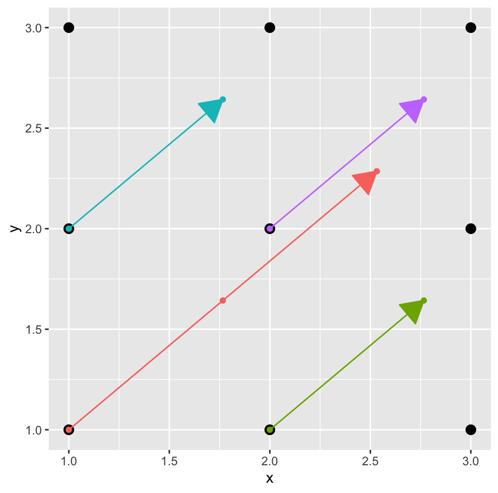
We want the coordinates of the dots along each of the colored arrows, and we want them all in two vectors, one for the x coordinates, and one for the y coordinates. These should look as follows:

path.x <- c(1.00,1.77,2.53,2.00,2.77,1.00,1.77,2.00,2.77)
path.y <- c(1.00,1.64,2.29,1.00,1.64,2.00,2.64,2.00,2.64)

Creating these vectors is not completely trivial, but essentially it boils down to the following steps:

sunazimuth <- 50 / 180 * pi
cossun <- cos(sunazimuth)
sinsun <- sin(sunazimuth)

coords.init <- expand.grid(x=1:2, y=1:2) # interior coordinates only
path.lengths <- c(3, 2, 2, 2)            # you need to calculate these

path.id <- rep(seq_len(nrow(coords.init)), path.lengths)
path.offsets <- sequence(path.lengths) - 1

rbind(path.id, path.offsets)

             [,1] [,2] [,3] [,4] [,5] [,6] [,7] [,8] [,9]
path.id         1    1    1    2    2    3    3    4    4
path.offsets    0    1    2    0    1    0    1    0    1

Each ray in figure 5 is represented by a path.id in this vector. The path.offsets values represent each step along the path. In our toy example only the ray starting at (1,1) is length three; all the others are length two.

Then it is just a matter of using some trig to compute the ray path coordinates:

path.x <- coords.init[path.id, 'x'] + path.offsets * sinsun
path.y <- coords.init[path.id, 'y'] + path.offsets * cossun

rbind(path.id, path.x=path.x, path.y=path.y) + 1e-6

        [,1] [,2] [,3] [,4] [,5] [,6] [,7] [,8] [,9]
path.id    1 1.00 1.00    2 2.00    3 3.00    4 4.00
path.x     1 1.77 2.53    2 2.77    1 1.77    2 2.77
path.y     1 1.64 2.29    1 1.64    2 2.64    2 2.64

For the figure 1, path.x and path.y are ~25MM elements long (550 x 505 x ~100 steps per path). While these are large vectors they are well within the bounds of what a modern system can handle.

The benefit of having every light path described by these two vectors is that we can call our height interpolation function without loops:

interp.heights <- faster_bilinear(heightmap, path.x, path.y)

The rest of the function is post processing to figure out what proportion of elevations clears the obstacles for each coordinate.

You can review the full function on github.

The astute reader will notice that the algorithm is no longer exactly the same. Instead of checking whether each azimuth-elevation path combination hits an obstacle, we just compute the maximum angular elevation of every point along the azimuth. This means we only call the height interpolation function once for each step along the path, instead of up to 25 times (once for each elevation). If the C++ function were re-written to do the same, it could be faster, although whether it is or not will depend on how often it gets to stop early under the existing structure.

Additionally, we do not technically have to compute the offset 0 values, but we left them in here for simplicity.

Conclusions

R will rarely be as fast as compiled code, but you can get close in most cases with some thought and care. That you have to be careful to produce fast R code is definitely a limitation of the language. It is offset by the hundreds of packages that already solve most slow-in-R problems with compiled code. Additionally, it is fairly easy to identify and replace bottle necks with compiled code. For example, for this case we could take the vectorized ray_shade2 function and replace just the faster_bilinear2 function with a compiled code function.

One final note: the algorithm here is interpolating the height maps between pixels. We also implement a simplified version that just uses the height of the nearest pixel in shadow::ray_shade3. It looks just as good and runs twice as fast (update: it does not work as well if you want smooth transitions between frames rendered at slightly different angles).

Appendix

Session Info

sessionInfo()

R version 3.6.2 (2019-12-12)
Platform: x86_64-apple-darwin15.6.0 (64-bit)
Running under: macOS Mojave 10.14.6

Matrix products: default
BLAS:   /Library/Frameworks/R.framework/Versions/3.6/Resources/lib/libRblas.0.dylib
LAPACK: /Library/Frameworks/R.framework/Versions/3.6/Resources/lib/libRlapack.dylib

locale:
[1] en_US.UTF-8/en_US.UTF-8/en_US.UTF-8/C/en_US.UTF-8/en_US.UTF-8

attached base packages:
[1] stats     graphics  grDevices utils     datasets  methods   base     

other attached packages:
[1] ggplot2_3.2.0

loaded via a namespace (and not attached):
 [1] Rcpp_1.0.1           knitr_1.23           magrittr_1.5        
 [4] tidyselect_0.2.5     munsell_0.5.0        colorspace_1.4-1    
 [7] R6_2.4.0             rlang_0.4.0          fansi_0.4.1         
[10] dplyr_0.8.3          stringr_1.4.0        tools_3.6.2         
[13] grid_3.6.2           gtable_0.3.0         xfun_0.8            
[16] withr_2.1.2          htmltools_0.3.6      assertthat_0.2.1    
[19] yaml_2.2.0           lazyeval_0.2.2       digest_0.6.20       
[22] tibble_2.1.3         crayon_1.3.4         bookdown_0.10       
[25] purrr_0.3.2          microbenchmark_1.4-6 glue_1.3.1          
[28] evaluate_0.14        rmarkdown_1.12       blogdown_0.12       
[31] labeling_0.3         stringi_1.4.3        compiler_3.6.2      
[34] pillar_1.4.2         scales_1.0.0         pkgconfig_2.0.2

Supporting Code

Code used in this blog post follows. It is in the order it needs to be run in to function, not in the order in which it is used by the post.

Code to load mountain elevation data:

# File originally from http://tylermw.com/data/dem_01.tif.zip
eltif <- raster::raster("~/Downloads/dem_01.tif")
eldat <- raster::extract(eltif,raster::extent(eltif),buffer=10000)
elmat1 <- matrix(eldat, nrow=ncol(eltif), ncol=nrow(eltif))

Code to generate figure 2:

sun <- 45                         # sunangle
els <- seq(-90, 90, length=25)    # elevations
elmat2 <- elmat1[, rev(seq_len(ncol(elmat1)))]  # rev columns for rayshader

t.for <- system.time(sh.for <- shadow::ray_shade1(elmat1, els, sun))
t.vec <- system.time(sh.vec <- shadow::ray_shade2(elmat1, els, sun))
t.cpp <- system.time(
  sh.cpp <- rayshader::ray_shade(elmat2, els, sun, lambert=FALSE)
)
# We compute the Julia time separately
types <- c('for', 'vectorized', 'cpp', 'julia')
time.dat <- data.frame(
  type=factor(types, levels=types),
  time.ratio=
    t.for['elapsed'] /
    c(t.for['elapsed'], t.vec['elapsed'], t.cpp['elapsed'],  7.4495)
)
ggplot(time.dat, aes(type, y=time.ratio)) + geom_col()

Code to generate figure 3:

dims <- lapply(dim(sh.cpp), seq_len)
df <- rbind(
   cbind(do.call(expand.grid, dims), z=c(sh.cpp), type='cpp'),
   cbind(do.call(expand.grid, dims), z=c(sh.vec), type='vec'),
   cbind(do.call(expand.grid, dims), z=c(sh.for), type='for')
)
df$type <- factor(df$type, levels=c('for', 'vec', 'cpp'))
plot_attr <- list(
  geom_raster(),
  scale_fill_gradient(low='#333333', high='#ffffff', guide=FALSE),
  ylab(NULL), xlab(NULL),
  scale_x_continuous(expand=c(0,0)),
  scale_y_continuous(expand=c(0,0)),
  theme(axis.text=element_text(size=6))
)
ggplot(df, aes(x=Var1, y=Var2, fill=z)) +
  facet_wrap(~type) + plot_attr

Code to generate figure 1:

ggplot(subset(df, type='vec'), aes(x=Var1, y=Var2, fill=z)) + plot_attr

Code to generate figure 5.

p
do.call(knitr::opts_chunk$set, old.opt)

Do Not Shade R