Error in library(treeprof): there is no package called 'treeprof'TL;DR

What do psychedelic triangles and chimeras have in common? Oddly the answer is “list data structures”. I discovered this while procrastinating from the side project that was my procrastination from my actual projects. Much to my surprise, shading triangles from vertex colors is faster with list data structures than with matrices and arrays. This despite the calculations involved being simple additions and multiplications on large atomic vectors.
As with everything in life there are caveats to this finding. It is primarily applicable to tall and skinny data sets, i.e. those with a very high ratio of observations to variables. It also requires some additional work over standard methods. Given that this type of data set is fairly common, it seems worth showing methods for working with list data structures. In my particular use case I saw speed improvements on the order of 2x to 4x.
If you are bored easily you might want to skip straight to the case study section of this post. If you like benchmarks and want an extensive review of list data structure manipulations, read on.
Matrices Are Slow?
Column Subsetting
Generally speaking matrices are amongst the R data structures that are fastest to operate on. After all, they are contiguous chunks of memory with almost no overhead. Unfortunately, they do come with a major limitation: any subset operation requires copying the data:
set.seed(1023)
n <- 1e5

M <- cbind(runif(n), runif(n), runif(n), runif(n))
D <- as.data.frame(M)
microbenchmark(M[,1:2], D[,1:2], times=25)
Unit: microseconds
expr min lq mean median uq max neval
M[, 1:2] 826 941.2 1839.3 1884.3 1934.0 7440.5 25
D[, 1:2] 16 17.3 35.2 26.8 48.4 89.7 25The data frame subset is much faster because R treats data frame columns as independent objects, so referencing an entire column does not require a copy. But data frames have big performance problems of their own. Let’s see what happens if we select columns and rows:
idx <- sample(seq_len(nrow(M)), n/2)
microbenchmark(M[idx,1:2], D[idx,1:2], times=25)
Unit: microseconds
expr min lq mean median uq max neval
M[idx, 1:2] 539 950 1337 1199 1276 7201 25
D[idx, 1:2] 8439 8861 9184 9336 9571 9729 25And its even worse if we have duplicate row indices:
idx2 <- c(idx, idx[1])
microbenchmark(M[idx2,1:2], D[idx2,1:2], times=25)
Unit: microseconds
expr min lq mean median uq max neval
M[idx2, 1:2] 807 1039 1311 1279 1587 1912 25
D[idx2, 1:2] 26549 27865 30621 28332 30479 61100 25Data frames have row names that are required to be unique and most of the row subsetting overhead comes from managing them.
Lists to the Rescue
With a little extra work you can do most of what you would normally do with a
matrix or data frame with a list. For example, to select “rows” in a list of
vectors, we use lapply to apply [ to each component vector:
L <- as.list(D)
str(L)
List of 4
$ V1: num [1:100000] 0.249 0.253 0.95 0.489 0.406 ...
$ V2: num [1:100000] 0.7133 0.4531 0.6676 0.651 0.0663 ...
$ V3: num [1:100000] 0.87 0.783 0.714 0.419 0.495 ...
$ V4: num [1:100000] 0.44475 0.90667 0.12428 0.00587 0.77874 ...sub.L <- lapply(L[1:2], '[', idx)
str(sub.L)List of 2
$ V1: num [1:50000] 0.178 0.326 0.179 0.349 0.587 ...
$ V2: num [1:50000] 0.5577 0.5571 0.4757 0.0805 0.9059 ...col_eq(sub.L, D[idx,1:2]) # col_eq compares values column by column[1] TRUEThis results in the same elements selected as with data frame or matrix
subsetting, except the result remains a list. You can see how col_eq compares
objects in the appendix.
Despite the explicit looping over columns this list based subsetting is comparable to matrix subsetting in speed:
microbenchmark(lapply(L[1:2], '[', idx), M[idx,1:2], D[idx,1:2], times=25)Unit: microseconds
expr min lq mean median uq max neval
lapply(L[1:2], "[", idx) 779 889 1270 1057 1184 7080 25
M[idx, 1:2] 817 983 1161 1199 1266 1582 25
D[idx, 1:2] 8208 9044 9188 9218 9626 9903 25And if we only index columns then the list is even faster than the data frame:
microbenchmark(L[1:2], M[,1:2], D[,1:2], times=25)Unit: nanoseconds
expr min lq mean median uq max neval
L[1:2] 755 1221 2936 1966 3447 9414 25
M[, 1:2] 1605476 1774546 1843095 1851509 1898917 2348802 25
D[, 1:2] 16906 19929 37796 33938 47832 76152 25Patterns in List Based Analysis
Row Subsetting
As we saw previously the idiom for subsetting “rows” from a list of equal length vectors is:
lapply(L, '[', idx)The lapply expression is equivalent to:
fun <- `[`
result <- vector("list", length(L))
for(i in seq_along(L)) result[[i]] <- fun(L[[i]], idx)
We use lapply to apply a function to each element of our list. In our case,
each element is a vector, and the function is the subset operator [. In R,
L[[i]][idx] and '['(L[[i]], idx) are equivalent as operators are really just
functions that R recognizes as functions at parse time.
Column Operations
We can extend the lapply principle to other operators and functions. To
multiply every column by two we can use:
microbenchmark(times=25,
  Matrix=  M * 2,
  List=    lapply(L, '*', 2)
)
Unit: microseconds
expr min lq mean median uq max neval
Matrix 657 2046 2441 2086 2161 9400 25
List 593 789 1995 2107 2219 8489 25This will work for any binary function. For unary functions we just omit the additional argument:
lapply(L, sqrt)We can also extend this to column aggregating functions:
microbenchmark(times=25,
  Matrix_sum=  colSums(M),
  List_sum=    lapply(L, sum),
  Matrix_min=  apply(M, 2, min),
  List_min=    lapply(L, min)
)
Unit: microseconds
expr min lq mean median uq max neval
Matrix_sum 490 579 593 587 604 749 25
List_sum 509 580 610 613 617 797 25
Matrix_min 5344 9225 9903 9688 10281 15839 25
List_min 919 1056 1100 1085 1143 1315 25In the matrix case we have the special colSums function that does all the
calculations in internal C code. Despite that it is no faster than the list
approach. And for operations without special column functions such as finding
the minimum by column we need to use apply, at which point the list approach
is much faster.
If we want to use different scalars for each column things get a bit more
complicated, particularly for the matrix approach. The most natural way to do
this with the matrix is to transpose and take advantage of column recycling.
For lists we can use Map:
vec <- 2:5
microbenchmark(times=25,
  Matrix= t(t(M) * vec),
  List=   Map('*', L, vec)
)
Unit: milliseconds
expr min lq mean median uq max neval
Matrix 4.28 4.67 7.01 7.54 7.88 13.43 25
List 1.22 1.43 2.72 2.94 3.05 8.65 25col_eq(t(t(M) * vec), Map('*', L, vec))[1] TRUEMap is a close cousin of mapply. It calls its first argument, in this case
the function *, with one element each from the subsequent arguments, looping
through the argument elements. We use Map instead of mapply because it is
guaranteed to always return a list, whereas mapply will simplify the result to
a matrix. It is equivalent to:
f <- `*`
result <- vector('list', length(vec))
for(i in seq_along(L)) result[[i]] <- f(L[[i]], vec[[i]])
There are some faster ways to do this with matrices, such as:
microbenchmark(times=25,
  Matrix=  M %*% diag(vec),
  List=    Map('*', L, vec)
)
Unit: milliseconds
expr min lq mean median uq max neval
Matrix 2.79 4.31 4.76 4.42 4.56 13.32 25
List 1.40 2.27 3.29 3.10 3.43 9.79 25col_eq(M %*% diag(vec), Map('*', L, vec))[1] TRUEBut even that is slower than the list approach, with the additional infirmities that it cannot be extended to other operators, and it works incorrectly if the data contains infinite values.
Map also allows us to operate pairwise on columns. Another way to compute the
square of our data might be:
microbenchmark(times=25,
  Matrix= M * M,
  List=   Map('*', L, L)
)
Unit: microseconds
expr min lq mean median uq max neval
Matrix 721 2091 2444 2151 2204 8172 25
List 686 1012 2076 2213 2298 8770 25col_eq(M * M, Map('*', L, L))[1] TRUERow-wise Operations
A classic row-wise operation is to sum values by row. This is easily done with
rowSums for matrices. For lists, we can use Reduce to collapse every column
into one:
microbenchmark(times=25,
  Matrix= rowSums(M),
  List=   Reduce('+', L)
)
Unit: microseconds
expr min lq mean median uq max neval
Matrix 1582 2504 3093 2759 3037 11973 25
List 595 1244 1362 1322 1707 2132 25col_eq(rowSums(M), Reduce('+', L))[1] TRUEMuch to my surprise Reduce is substantially faster, despite explicitly looping
through the columns. From informal testing Reduce has an edge up to ten
columns or so. This may be because rowSums will use long double to store
the interim results of the row sums, whereas + will just add double values
directly, with some loss of precision as a result.
Reduce collapses the elements of the input list by repeatedly applying a
binary function to turn two list elements into one. Reduce is equivalent to:
result <- numeric(length(L[[1]]))
for(l in L) result <- result + l
An additional advantage of the Reduce approach is you can use any binary
function for the row-wise aggregation.
List to Matrix and Back
R is awesome because it adopts some of the better features of functional languages and list based languages. For example, the following two statements are equivalent:
ML1 <- cbind(x1=L[[1]], y1=L[[2]], x2=L[[3]], y2=L[[4]])
ML2 <- do.call(cbind, L)
Proof:
col_eq(ML1, ML2)[1] TRUEcol_eq(ML1, M)[1] TRUEThe blurring of calls, lists, data, and functions allows for very powerful
manipulations of list based data. In this case, do.call(cbind, LIST) will
transform any list containing equal length vectors into a matrix, irrespective
of how many columns it has.
To go in the other direction:
LM <- lapply(seq_len(ncol(M)), function(x) M[,x])
col_eq(L, LM)
[1] TRUEYou could use split but it is much slower.
More on do.call
List based analysis works particularly well with do.call and functions that
use ... parameters:
microbenchmark(times=25,
  List=   do.call(pmin, L),
  Matrix= pmin(M[,1],M[,2],M[,3],M[,4])
)
Unit: milliseconds
expr min lq mean median uq max neval
List 2.64 3.06 3.12 3.16 3.22 3.61 25
Matrix 4.80 7.27 7.90 7.44 7.73 15.97 25The expression is both easier to type, and faster!
There are a couple of “gotchas” with do.call, particularly if you try
to pass quoted language as part of the argument list (e.g. quote(a + b)). If
you are just using normal R data objects then the one drawback that I am
aware of is that the call stack can get messy if you ever invoke traceback()
or sys.calls() from a function called by do.call. An issue related to this
is that do.call calls that error can become very slow. So long as you are
sure the do.call call is valid there should be no problem.
Remember that data frames are lists, so you can do things like:
do.call(pmin, iris[-5])High Dimensional Data
Matrices naturally extend to arrays in high dimensional data. Imagine we wish to track triangle vertex coordinates in 3D space. We can easily set up an array structure to do this:
verts <- 3
dims <- 3
V <- runif(n * verts * dims)
tri.A <- array(
  V, c(n, verts, dims),
  dimnames=list(NULL, vertex=paste0('v', seq_len(verts)), dim=c('x','y','z'))
)
tri.A[1:2,,]
, , dim = x
vertex
v1 v2 v3
[1,] 0.322 0.119 0.965
[2,] 0.130 0.540 0.643
, , dim = y
vertex
v1 v2 v3
[1,] 0.989 0.400 0.346
[2,] 0.935 0.338 0.754
, , dim = z
vertex
v1 v2 v3
[1,] 0.551 0.260 0.560
[2,] 0.232 0.543 0.564How do we do this with lists? Well, it turns out that you can make list-matrices and list-arrays. First we need to manipulate our data little as we created it originally for use with an array:
MV <- matrix(V, nrow=n)
tri.L <- lapply(seq_len(verts * dims), function(x) MV[,x])
Then, we just add dimensions:
dim(tri.L) <- tail(dim(tri.A), -1)
dimnames(tri.L) <- tail(dimnames(tri.A), -1)
tri.L
dim
vertex x y z
v1 Numeric,100000 Numeric,100000 Numeric,100000
v2 Numeric,100000 Numeric,100000 Numeric,100000
v3 Numeric,100000 Numeric,100000 Numeric,100000class(tri.L)[1] "matrix" "array" typeof(tri.L)[1] "list"A chimera! tri.L is a list-matrix. While this may seem strange if you haven’t
come across one previously, the list matrix and 3D array are essentially
equivalent:
head(tri.A[,'v1','x'])[1] 0.322 0.130 0.587 0.785 0.967 0.448head(tri.L[['v1','x']])[1] 0.322 0.130 0.587 0.785 0.967 0.448An example operation might be to find the mean value of each coordinate for each vertex:
colMeans(tri.A) dim
vertex x y z
v1 0.5 0.500 0.500
v2 0.5 0.499 0.500
v3 0.5 0.500 0.501apply(tri.L, 1:2, do.call, what=mean) dim
vertex x y z
v1 0.5 0.500 0.500
v2 0.5 0.499 0.500
v3 0.5 0.500 0.501apply with the second argument set to 1:2 is equivalent to:
MARGIN <- 1:2
result <- vector('list', prod(dim(tri.L)[MARGIN]))
dim(result) <- dim(tri.L)[MARGIN]
fun <- do.call
for(i in seq_len(nrow(tri.L)))
  for(j in seq_len(ncol(tri.L)))
    result[i, j] <- fun(what=mean, tri.L[i, j])
We use do.call because tri.L[i, j] is a list, and we wish to call mean
with the contents of the list, not the list itself. We could also have used a
function like function(x) mean(x[[1]]) instead of do.call.
We’ll be using list matrices in the next section.
A Case Study
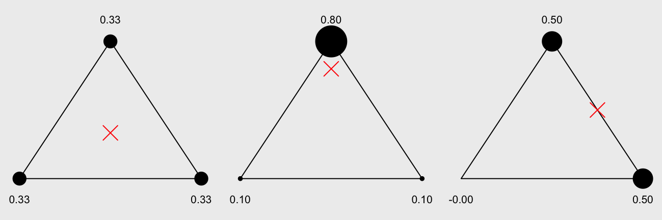
One of my side projects required me to implement barycentric coordinate conversions. You can think of barycentric coordinates of a point in a triangle as the weights of the vertices that cause the triangle to balance on that point.
We show here three different points (red crosses) with the barycentric coordinates associated with each vertex. The size of the vertex helps visualize the “weights”:
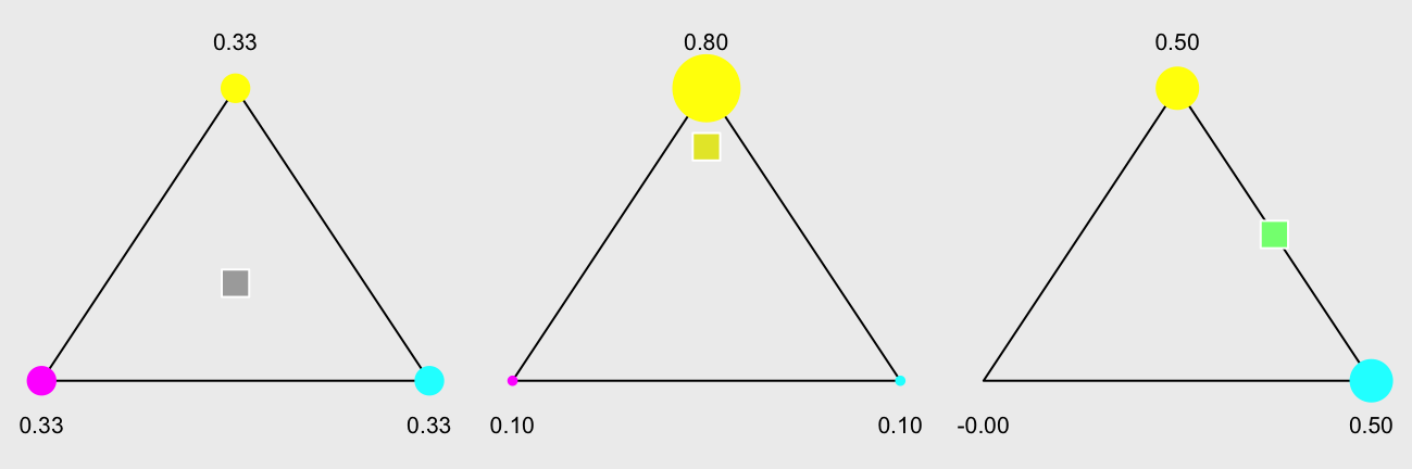
This is useful if we want to interpolate values from the vertices to points in the triangle. Here we interpolate a color for a point in a triangle from the colors of the vertices of that triangle:
The formula for converting cartesian coordinates to Barycentric is:
\[\lambda_1 = \frac{(y_2 - y_3)(x - x_3) + (x_3 - x_2)(y - y_3)}{(y_2 - y_3)(x_1 - x_3) + (x_3 - x_2)(y_1 - y_3)}\\ \lambda_2 = \frac{(y_3 - y_1)(x - x_3) + (x_1 - x_3)(y - y_3)}{(y_2 - y_3)(x_1 - x_3) + (x_3 - x_2)(y_1 - y_3)}\\ \lambda_3 = 1 - \lambda_1 - \lambda_2\]
You can see that whatever the data structure is, we will be using a lot of
column subsetting for this calculation. We implement bary_A and bary_L to
convert Cartesian coordinates to barycentric using array and list-matrix data
structures respectively. Since both of these are direct translations of
the above formulas, we relegate them to the code
appendix. We will use them to shade every point of
our triangle with the weighted color of the vertices.
First, the data (defined in the appendix):
str(point.L) # every point we want to compute colorList of 2
$ x: num [1:79946] 0 0.00251 0.00501 0.00752 0.01003 ...
$ y: num [1:79946] 0.067 0.067 0.067 0.067 0.067 ...vertex.L # list-matrix! Data
V x y r g b
v1 Numeric,79946 Numeric,79946 Numeric,79946 Numeric,79946 Numeric,79946
v2 Numeric,79946 Numeric,79946 Numeric,79946 Numeric,79946 Numeric,79946
v3 Numeric,79946 Numeric,79946 Numeric,79946 Numeric,79946 Numeric,79946The vertex.L list-matrix has the x, y coordinates and the red, green, and blue
color channel vales of the triangle associated with each point. In this
particular case it happens to be the same triangle for every point, so we could
have used a single instance of the triangle. The generalization needs to
allow for many triangles with a small and varying number of points per triangle,
and to handle that efficiently in R we need to match each point to its own
triangle.
And the shading function:
v_shade_L <- function(p, v) {
  ## 1) compute barycentric coords
  bc <- bary_L(p, v)
  ## 2) for each point, weight vertex colors by bary coords
  clr.raw <- apply(v[, c('r','g','b')], 2, Map, f="*", bc)
  ## 3) for each point-colorchannel, sum the weighted values
  lapply(clr.raw, Reduce, f="+")
}
Step 1) is carried out by bary_L, which is a simple adaptation of
the barycentric conversion formulas. Step 2) is the most
complicated. To understand what’s going on we need to look at the two data
inputs to apply, which are:
v[, c('r','g','b')] Data
V r g b
v1 Numeric,79946 Numeric,79946 Numeric,79946
v2 Numeric,79946 Numeric,79946 Numeric,79946
v3 Numeric,79946 Numeric,79946 Numeric,79946str(bc)List of 3
$ : num [1:79946] 1 0.997 0.995 0.992 0.99 ...
$ : num [1:79946] 0 0 0 0 0 0 0 0 0 0 ...
$ : num [1:79946] 0 0.00251 0.00501 0.00752 0.01003 ...In:
clr.raw <- apply(v[, c('r','g','b')], 2, Map, f="*", bc)We ask apply to call Map for each column of v[, c('r','g','b')]. The
additional arguments f='*' and bc are passed on to Map such that, for the
first column, the Map call is:
Map('*', v[,'r'], bc)v[,'r'] is a list with the red color channel values for each of the three
vertices for each of the points in our data:
str(v[,'r'])List of 3
$ v1: num [1:79946] 1 1 1 1 1 1 1 1 1 1 ...
$ v2: num [1:79946] 1 1 1 1 1 1 1 1 1 1 ...
$ v3: num [1:79946] 0 0 0 0 0 0 0 0 0 0 ...bc is a list of the barycentric coordinates of each point which we will use as
the vertex weights when averaging the vertex colors to point colors:
str(bc)List of 3
$ : num [1:79946] 1 0.997 0.995 0.992 0.99 ...
$ : num [1:79946] 0 0 0 0 0 0 0 0 0 0 ...
$ : num [1:79946] 0 0.00251 0.00501 0.00752 0.01003 ...The Map call is just multiplying each color value by its vertex weight.
apply will repeat this over the three color channels giving us the barycentric
coordinate-weighted color channel values for each point:
str(clr.raw)List of 3
$ r:List of 3
..$ v1: num [1:79946] 1 0.997 0.995 0.992 0.99 ...
..$ v2: num [1:79946] 0 0 0 0 0 0 0 0 0 0 ...
..$ v3: num [1:79946] 0 0 0 0 0 0 0 0 0 0 ...
$ g:List of 3
..$ v1: num [1:79946] 0 0 0 0 0 0 0 0 0 0 ...
..$ v2: num [1:79946] 0 0 0 0 0 0 0 0 0 0 ...
..$ v3: num [1:79946] 0 0.00251 0.00501 0.00752 0.01003 ...
$ b:List of 3
..$ v1: num [1:79946] 1 0.997 0.995 0.992 0.99 ...
..$ v2: num [1:79946] 0 0 0 0 0 0 0 0 0 0 ...
..$ v3: num [1:79946] 0 0.00251 0.00501 0.00752 0.01003 ...Step 3) collapses the weighted values into (r,g,b) triplets for each point:
str(lapply(clr.raw, Reduce, f="+"))List of 3
$ r: num [1:79946] 1 0.997 0.995 0.992 0.99 ...
$ g: num [1:79946] 0 0.00251 0.00501 0.00752 0.01003 ...
$ b: num [1:79946] 1 1 1 1 1 1 1 1 1 1 ...And with the colors we can render our fully shaded triangle (see appendix for
plot_shaded):
color.L <- v_shade_L(point.L, vertex.L)
plot_shaded(point.L, do.call(rgb, color.L))
The corresponding function in array format looks very similar to the list one:
v_shade_A <- function(p, v) {
  ## 1) compute barycentric coords
  bc <- bary_A(p, v)
  ## 2) for each point, weight vertex colors by bary coords
  v.clrs <- v[,,c('r','g','b')]
  clr.raw <- array(bc, dim=dim(v.clrs)) * v.clrs
  ## 3) for each point-colorchannel, sum the weighted values
  rowSums(aperm(clr.raw, c(1,3,2)), dims=2)
}
For a detailed description of what it is doing see the appendix. The take-away for now is that every function in the array implementation is fast in the sense that all the real work is done in internal C code.
The data are also similar, although they are in matrix and array format instead of list and matrix-list:
str(point.A) num [1:79946, 1:2] 0 0.00251 0.00501 0.00752 0.01003 ...
- attr(*, "dimnames")=List of 2
..$ : NULL
..$ : chr [1:2] "x" "y"str(vertex.A) num [1:79946, 1:3, 1:5] 0 0 0 0 0 0 0 0 0 0 ...
- attr(*, "dimnames")=List of 3
..$ : NULL
..$ V : chr [1:3] "v1" "v2" "v3"
..$ Data: chr [1:5] "x" "y" "r" "g" ...Both shading implementations produce the same result:
color.A <- v_shade_A(point.A, vertex.A)
col_eq(color.L, color.A)
[1] TRUEYet, the list based shading is substantially faster:
microbenchmark(times=25,
  v_shade_L(point.L, vertex.L),
  v_shade_A(point.A, vertex.A)
)
Unit: milliseconds
expr min lq mean median uq max neval
v_shade_L(point.L, vertex.L) 11.9 14.3 17.6 15.3 20.9 31.4 25
v_shade_A(point.A, vertex.A) 57.9 63.4 72.9 70.1 78.6 131.3 25We can get a better sense of where the speed differences are coming from by
looking at the profile data using treeprof:
treeprof(v_shade_L(point.L, vertex.L))Error in treeprof(v_shade_L(point.L, vertex.L), target.time = 1): could not find function "treeprof"treeprof(v_shade_A(point.A, vertex.A))Error in treeprof(v_shade_A(point.A, vertex.A), target.time = 1): could not find function "treeprof"Most of the time difference is in the bary_L vs bary_A
functions that compute the barycentric coordinates. You can also tell that
because almost all the time in the bary_* functions is “self” time (the second
column in the profile data) that this time is all spent doing primitive /
internal operations.
Step 2) takes about the same amount of time for both the list-matrix and array
methods (the apply call for v_shade_L and the array call for v_shade_A,
but step 3) is also much faster for the list approach because with the
array approach we need to permute the dimensions so we can use rowSums (more
details in the appendix).
Conclusion
If your data set is tall and skinny, list data structures can improve performance without compiled code or additional external dependencies. Most operations are comparable in speed whether done with matrices or lists, but key operations are faster and that make some tasks noticeably more efficient.
One trade-off is that the data manipulation can be more difficult with lists,
but for code in a package the extra work may be justified. Additionally, this
is not always true: patterns like do.call(fun, list) simplify tasks that
can be awkward with matrices.
Questions? Comments? @ me on Twitter.
Appendix
Session Info
sessionInfo()R version 4.0.2 (2020-06-22)
Platform: x86_64-apple-darwin17.0 (64-bit)
Running under: macOS Mojave 10.14.6
Matrix products: default
BLAS: /Library/Frameworks/R.framework/Versions/4.0/Resources/lib/libRblas.dylib
LAPACK: /Library/Frameworks/R.framework/Versions/4.0/Resources/lib/libRlapack.dylib
locale:
[1] en_US.UTF-8/en_US.UTF-8/en_US.UTF-8/C/en_US.UTF-8/en_US.UTF-8
attached base packages:
[1] stats graphics grDevices utils datasets methods base
other attached packages:
[1] microbenchmark_1.4-7
loaded via a namespace (and not attached):
[1] Rcpp_1.0.4.6 bookdown_0.18 fansi_0.4.1 digest_0.6.25
[5] magrittr_1.5 evaluate_0.14 blogdown_0.18 rlang_0.4.7
[9] stringi_1.4.6 rmarkdown_2.1 tools_4.0.2 stringr_1.4.0
[13] xfun_0.13 yaml_2.2.1 compiler_4.0.2 htmltools_0.4.0
[17] knitr_1.28 Column Equality
col_eq <- function(x, y) {
  if(is.matrix(x)) x <- lapply(seq_len(ncol(x)), function(z) x[, z])
  if(is.matrix(y)) y <- lapply(seq_len(ncol(y)), function(z) y[, z])
  # stopifnot(is.list(x), is.list(y))
  all.equal(x, y, check.attributes=FALSE)
}
Barycentric Conversions
## Conversion to Barycentric Coordinates; List-Matrix Version

bary_L <- function(p, v) {
  det <-  (v[[2,'y']]-v[[3,'y']])*(v[[1,'x']]-v[[3,'x']]) +
          (v[[3,'x']]-v[[2,'x']])*(v[[1,'y']]-v[[3,'y']])

  l1 <- (
          (v[[2,'y']]-v[[3,'y']])*(  p[['x']]-v[[3,'x']]) +
          (v[[3,'x']]-v[[2,'x']])*(  p[['y']]-v[[3,'y']])
        ) / det
  l2 <- (
          (v[[3,'y']]-v[[1,'y']])*(  p[['x']]-v[[3,'x']]) +
          (v[[1,'x']]-v[[3,'x']])*(  p[['y']]-v[[3,'y']])
        ) / det
  l3 <- 1 - l1 - l2
  list(l1, l2, l3)
}
## Conversion to Barycentric Coordinates; Array Version
bary_A <- function(p, v) {
det <- (v[,2,'y']-v[,3,'y'])*(v[,1,'x']-v[,3,'x']) +
(v[,3,'x']-v[,2,'x'])*(v[,1,'y']-v[,3,'y'])
l1 <- (
(v[,2,'y']-v[,3,'y']) * (p[,'x']-v[,3,'x']) +
(v[,3,'x']-v[,2,'x']) * (p[,'y']-v[,3,'y'])
) / det
l2 <- (
(v[,3,'y']-v[,1,'y']) * (p[,'x']-v[,3,'x']) +
(v[,1,'x']-v[,3,'x']) * (p[,'y']-v[,3,'y'])
) / det
l3 <- 1 - l1 - l2
cbind(l1, l2, l3)
}In reality we could narrow some of the performance difference between these two
implementations by avoiding repeated subsets of the same data. For example,
v[,3,'y'] is used several times, and we could have saved that subset to
another variable for re-use.
Plotting
plot_shaded <- function(p, col, v=vinit) {
  par(bg='#EEEEEE')
  par(xpd=TRUE)
  par(mai=c(.25,.25,.25,.25))
  plot.new()

  points(p, pch=15, col=col, cex=.2)
  polygon(v[,c('x', 'y')])
  points(
    vinit[,c('x', 'y')], pch=21, cex=5,
    bg=rgb(apply(v[, c('r','g','b')], 2, unlist)), col='white'
  )
}
Array Shading
v_shade_A <- function(p, v) {
  ## 1) compute barycentric coords
  bc <- bary_A(p, v)
  ## 2) for each point, weight vertex colors by bary coords
  v.clrs <- v[,,c('r','g','b')]
  clr.raw <- array(bc, dim=dim(v.clrs)) * v.clrs
  ## 3) for each point-colorchannel, sum the weighted values
  rowSums(aperm(clr.raw, c(1,3,2)), dims=2)
}
There are two items that may require additional explanation in v_shade_A.
First, as part of step 2) we use:
array(bc, dim=dim(v.clrs)) * v.clrsOur problem is that we need to multiply the vertex weights in bc with the
v.clrs color channel values, but they do not conform:
dim(bc)[1] 79946 3dim(v.clrs)[1] 79946 3 3Since we use the same weights for each color channel, it is just a matter of
recycling the bc matrix once for each channel. Also, since the color channel
is the last dimension we can just let array recycle the data to fill out the
product of the vertex data dimensions:
dim(array(bc, dim=dim(v.clrs)))[1] 79946 3 3This is reasonably fast, but not completely ideal since it does mean we need to
allocate a memory chunk the size of v.clrs. Ideally R would internally
recycle the bc matrix as it recycles vectors in situations like matrix(1:4, 2) * 1:2, but that is not how it is.
The other tricky bit is part of step 3):
rowSums(aperm(clr.raw, c(1,3,2)), dims=2)We ask rowSums to preserve the first two dimensions of the array with
dims=2. The other dimensions are collapsed by summing the values that overlap
in the first two. Unfortunately, we can only specify adjacent dimensions to
preserve with rowSums. As a result we permute the data with aperm so that
the point and color channel dimensions can be the first two and thus be
preserved.
There may be clever ways to better structure the data to minimize the number of copies we make.
Data
## Define basic triangle vertex position and colors

height <- sin(pi/3)
v.off <- (1 - height) / 2
vinit <- cbind(
  x=list(0, .5, 1), y=as.list(c(0, height, 0) + v.off),
  r=list(1, 1, 0), g=list(0,1,1), b=list(1,0,1)
)
## Sample points within the triangles

p1 <- list(x=.5, y=tan(pi/6) * .5 + v.off)
p2 <- list(x=.5, y=sin(pi/3) * .8 + v.off)
p3 <- list(x=cos(pi/6)*sin(pi/3), y=sin(pi/3) * .5 + v.off)

## Generate n x n sample points within triangle; here we also expand the
## vertex matrix so there is one row per point, even though all points are
## inside the same triangle.  In our actual use case, there are many
## triangles with a handful of points within each triangle.

n <- 400
rng.x <- range(unlist(vinit[,'x']))
rng.y <- range(unlist(vinit[,'y']))
points.raw <- expand.grid(
  x=seq(rng.x[1], rng.x[2], length.out=n),
  y=seq(rng.y[1], rng.y[2], length.out=n),
  KEEP.OUT.ATTRS=FALSE
)
vp <- lapply(vinit, '[', rep(1, nrow(points.raw)))
dim(vp) <- dim(vinit)
dimnames(vp) <- dimnames(vinit)

## we're going to drop the oob points for the sake of clarity, one
## nice perk of barycentric coordinates is that negative values indicate
## you are out of the triangle.

bc.raw <- bary_L(points.raw, vp)
inbounds <- Reduce('&', lapply(bc.raw, '>=', 0))

## Make a list-matrix version of the data

point.L <- lapply(points.raw, '[', inbounds)
vertex.L <- lapply(vp, '[', inbounds)
dim(vertex.L) <- dim(vp)
dimnames(vertex.L) <- list(V=sprintf("v%d", 1:3), Data=colnames(vp))

## Generate an array version of the same data

point.A <- do.call(cbind, point.L)
vertex.A <- array(
  unlist(vertex.L), c(sum(inbounds), nrow(vertex.L), ncol(vertex.L)),
  dimnames=c(list(NULL), dimnames(vertex.L))
)