Vectorize The Absolute $#!+ Out Of This

I wish I could tell you that I carefully figured out all the intricacies of the RTIN algorithm before I set off on my initial vectorization attempt, that I didn’t waste hours going cross-eyed at triangles poorly drawn on scraps of paper, and that I didn’t produce algorithms which closer inspection showed to be laughably incorrect. Instead I’ll have to be content with telling you that I did get this to work eventually.

It turns out that that truly understanding an algorithm you’re trying to re-implement is fairly important. Who woulda thunk?

Some Triangles Are More Equal Than Others

The root cause of my early failures at re-implementing @mourner’s martini is that there are more different types of triangles than is obvious at first glance. They are all isoceles right angled triangles, but there are eight possible orientations and each orientation is only valid at specific locations in the mesh.

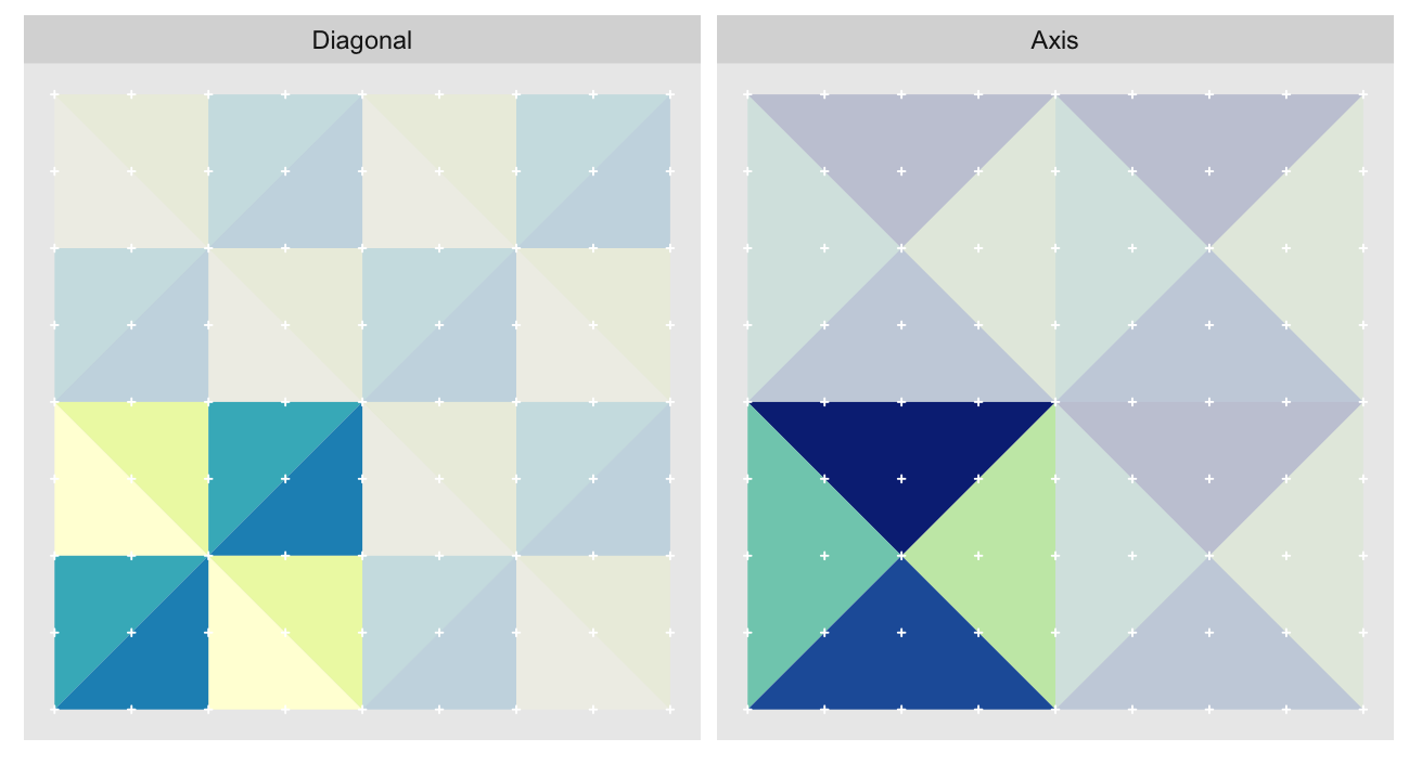
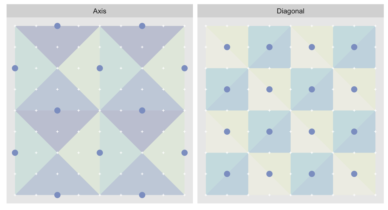
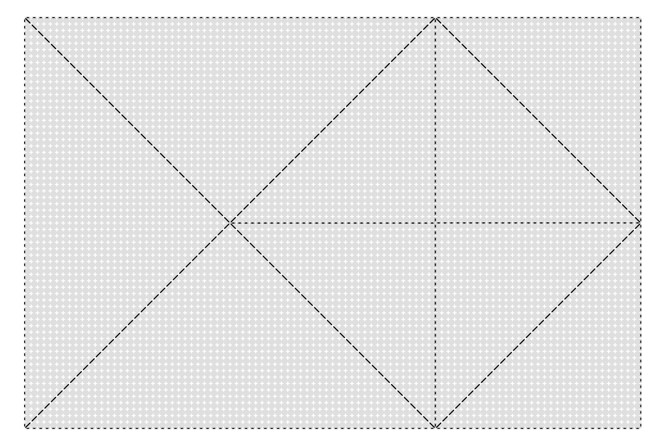
The orientations can be split into two groups of four, with the groups alternating between approximation levels. Here we show the orientations for the 2nd and 3rd most granular levels of a 9 x 9 grid¹. The triangles are colored by orientation. Because we’re very imaginative we’ll call the group diagonal hypotenuses “Diagonal”, and the one with vertical/horizontal ones “Axis”:

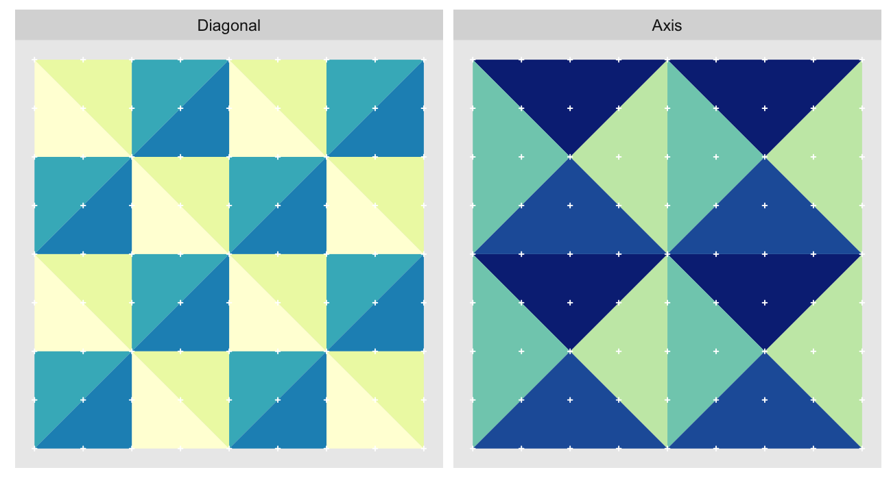
The “Axis” triangulation, the one with vertical and horizontal hypotenuses, has just one tiling pattern. A particular triangle “shape” (a specific color in the plot above) must always be arranged in the same way relative to the other shapes that share the vertex opposite their hypotenuses. Any other arrangement would prevent us from fully tiling the grid without breaking up triangles.

On the other hand the “Diagonal” triangulation, has multiple possible tilings:

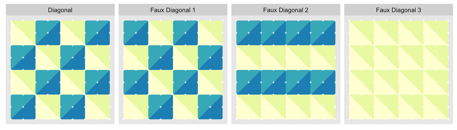
We show just three alternate tilings, although there are $2^{16}$. All of them perfectly cover the grid with equal sized triangles. “Faux Diagonal 1” is even a pretty convincing replica. Unfortunately only one of them fits exactly into the next level of coarseness, “Axis” shown previously, seen here in a green outline:

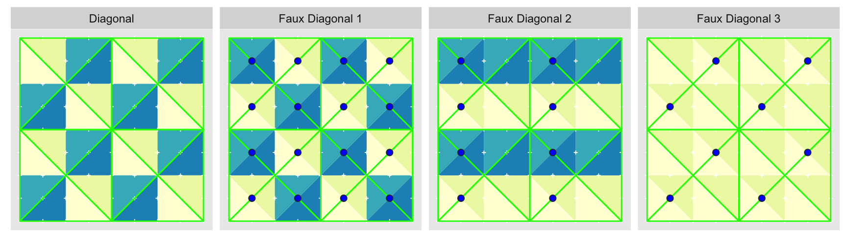
It is only with “Diagonal” that every edge of the parent approximation level completely overlaps with edges of the child. Every other arrangement has at least one parent edge crossing a hypotenuse of a child triangle. These crossings are what the blue circles highlight. Ironically, the best looking fake is the worst offender.

Herein lies the beauty of @mourner’s implementation; by deriving child triangles from splitting the parent ones, we guarantee that the child triangles will conform to the parents. As I learned painfully no such guarantees apply when we compute the coordinates directly.

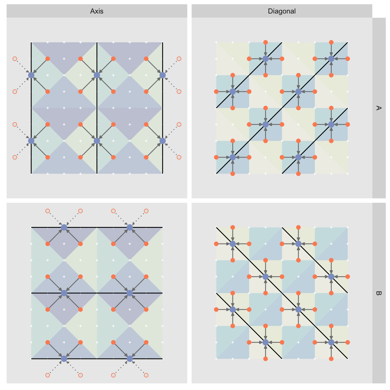
There are many ways to solve this vectorization problem, but the simplest I could come up with was to treat it as a tiling task. The idea is to define the smallest tessellating patterns that extend to the correct layout. These patterns can then be repeated as needed in internally vectorized manner². This is what they look like for our 9 x 9 example:

Unfortunately this is insufficient. We must also for each triangle hypotenuse midpoint track their children so that we may carry over their errors. One nice benefit of the tessellating pattern is that if we define the parent-child relationship for the simple tile, we can copy that relationship along with the rest of the tile. In fact, we don’t actually care about the triangles. What we actually want are the hypotenuses (black lines), their midpoints, endpoints, and the corresponding child hypotenuse midpoints. The parent/child relation is shown with the arrows:

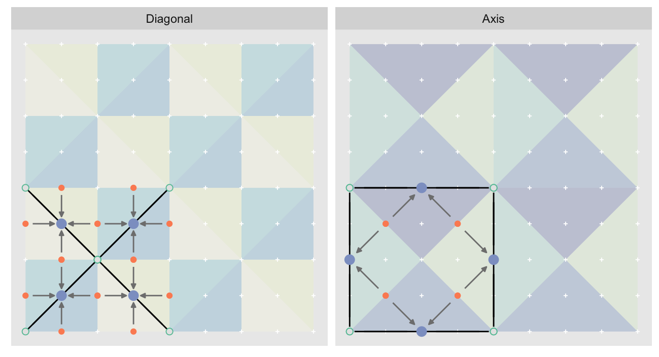
Recall: we are trying to compute the error in approximating the hypotenuse midpoints as the mean of the endpoints, while carrying over error of the child midpoint approximations. Notice how the midpoints of the “Diagonal” layer become the child midpoints in the “Axis” layer.

See RTINI Part I for additional details on the algorithm.

Now Just Tile the Rest of the $#!+ing Map

Great, we have a concept for how we might parallelize the computation of critical coordinates, but how exactly do we do this in an efficiently vectorized manner? There are likely many ways, but what we’ll do is use “linearized” indices into the matrix. These indices treat the matrix as if it were a vector. The first step is to generate the template tile, which we will do with init_offsets, presented here in simplified form³:

init_offsets <- function(i, j, n, layers) {
  o <- if(j == 'axis') offset.ax else offset.dg    # raw coords
  o <- o * 2^(i - 1)                               # scale
  array(o[,1,] + o[,2,] * (n + 1) + 1, dim(o)[-2]) # x/y -> id
}

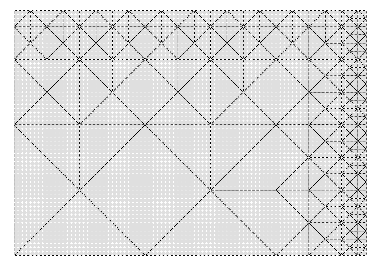
offset.ax and offset.dg are arrays that contain manually computed x/y coordinates for each of the points in the template tile. init_offsets scales those to the appropriate size for the layer and collapses them to “linearized” coordinates⁴. Here is the “Diagonals” map with the grid points labeled with their “linearized” coordinates and the key points of the template tile in the same colors as previously:

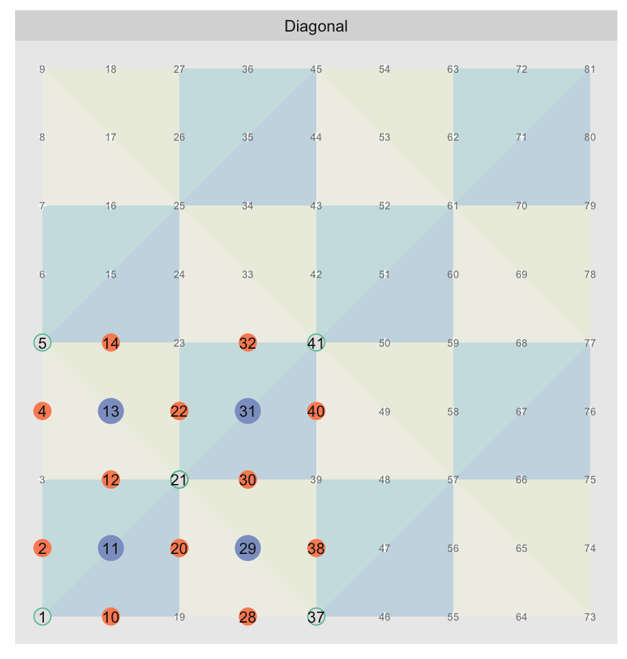
init_offsets produces the coordinates for the template tile:

n <- nrow(map)
init_offsets(i=1, j='diag', n=(n - 1), layers=log2(n - 1))

     [,1] [,2] [,3] [,4] [,5] [,6] [,7]
[1,]    1   21   11  20   10    2   12 
[2,]    5   21   13  22   14   12    4 
[3,]   21   37   29  38   30   28   20 
[4,]   21   41   31  40   30   22   32 

There are repeats as some points are shared across triangles. For example point 21 is a hypotenuse endpoint to all triangles. We can’t just drop the duplicates as the above structure tracks the midpoint by row, and we need the child midpoints and endpoints associated with each of them.

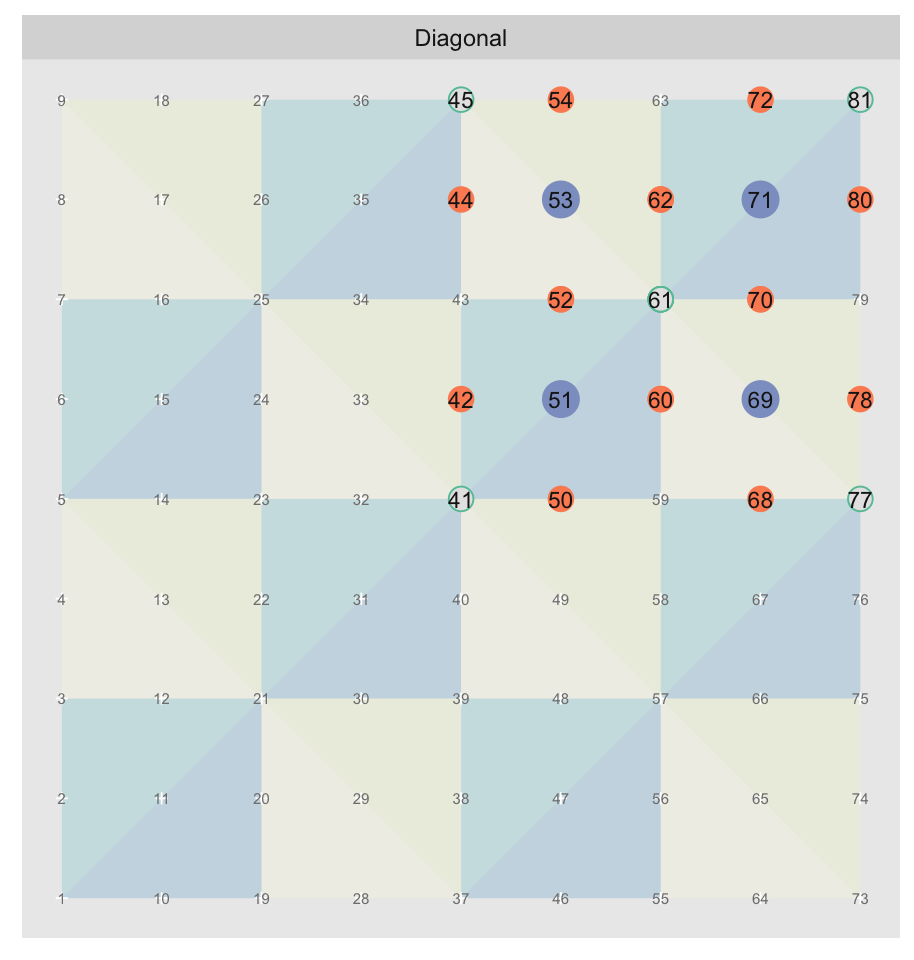
We can shift “linearized” coordinates, by simple arithmetic. For example, adding one to a coordinate will move it up one row⁵. Adding nrow(map) will shift the coordinates by one column. So for example:

init_offsets(i=1, j='diag', n=n - 1, layers=log2(8)) + 4 + 4 * n

Would shift the template four rows and four columns to produce:

Tiling is then just a matter of copying and shifting the template tile.

Action!

Let’s look at this in action with the next grid size up for effect. As we did in the prior post we’ll track the coordinates in the left panel side (both “Diagonal” and “Axis”, alternating), and the computed mesh approximation errors in the right hand panel:

For each “layer”, we start with a repeatable template sized to the layer. We then fill a column with it, then the rest of the surface, and finally we compute errors. Here is the same thing as a flipbook with code so we can see how it’s actually done. Remember that in these flipbooks the state shown is immediately after the highlighted line is evaluated. We’ll focus on the second set of layers:

o, as shown in the first frame⁶ contains the offsets that represent the template tile. These offsets are generated by init_offsets, which we reviewed earlier.

Since the tile coordinates are linearized we can shift them by repeating the template while adding different offsets to each repeat:

seq.r <- (seq_len(tile.n) - 1) * n / tile.n
o <- rep(o, each=tile.n) + seq.r

We first repeat the template tile four times (tile.n), and then shift them by seq.r:

seq.r

[1]  0  4  8 12

Due to how we repeat o each value of seq.r will be recycled for every value of o. The result is to copy the template tile to fill the column. Similarly we can fill the rest of the surface by repeating and shifting the column:

o <- rep(o, each=tile.n) + seq.r * (n + 1)

The points are arranged by type in the original offset list so we can easily subset for a particular type of point from the repeated tile set:

o.m <- o[o.i + 2 * o.len]    # midpoint coordinate
o.b <- o[o.i + o.len]        # 1st hypotenuse endpoint coordinate
o.a <- o[o.i]                # 2nd hypotenuse endpoint coordinate

This is how the visualization knows to color the points as the point type is never explicitly stated in the code. Additionally, the relative positions of parents and children are also preserved.

After calculating the errors we must record the maximum of the error and child errors. This includes the following seemingly funny business:

err.val <- do.call(pmax, err.vals)
err.ord <- order(err.val)                  # <<< Order
errors[o.m[err.ord]] <- err.val[err.ord]

This is necessary because for “Axis” tiling the same midpoints may be updated by two different tiles as is the case here when we fill a column:

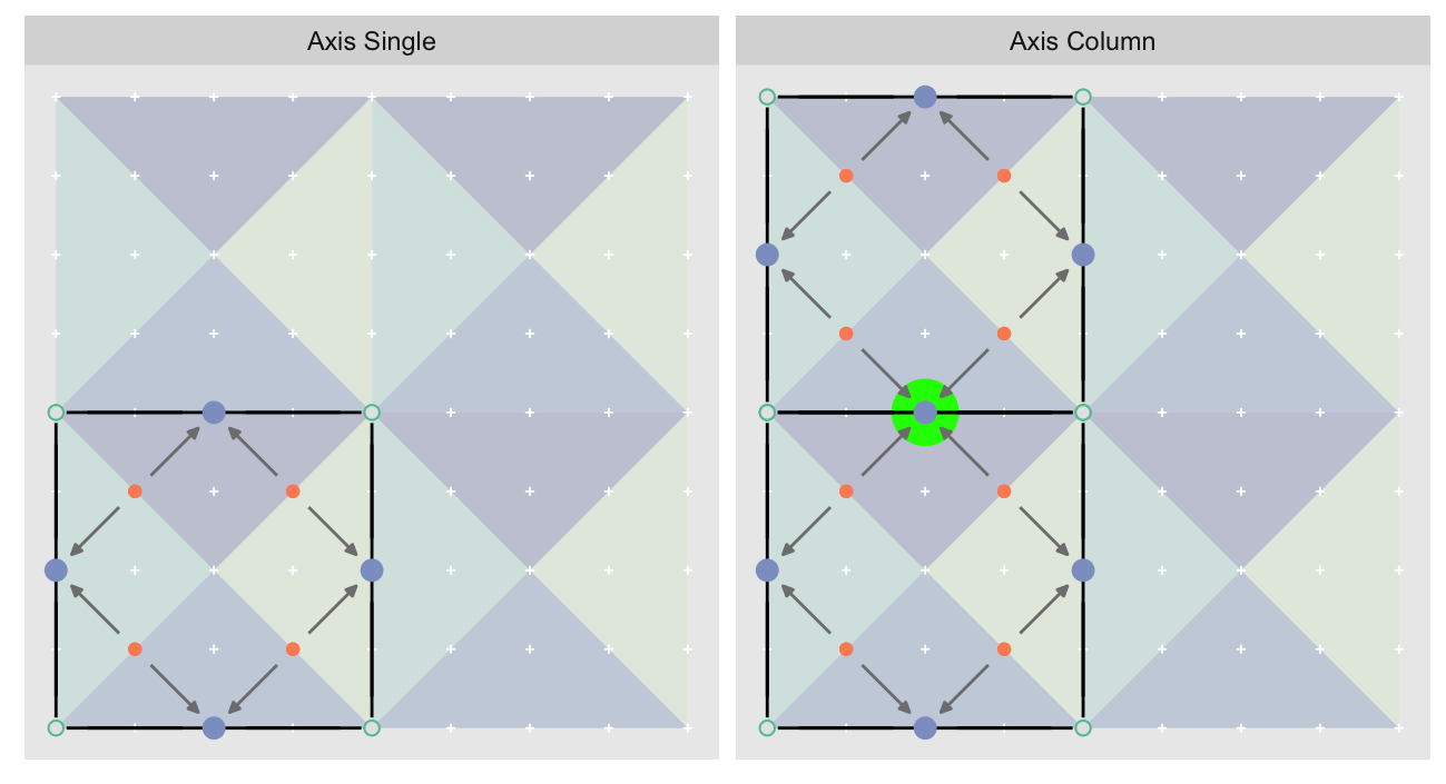
The midpoint highlighted in green is at the overlap of two tiles, so we are carrying over errors from children in different tiles. If we did not order err.val prior to final insertion into the error matrix we risk a lesser error from one tile overwriting a larger error from another. This issue afflicts all the non-peripheral midpoints in the “Axis” tile arrangement⁷.

The full code of this implementation is available in the appendix.

Loopy Vectorization?

Hold on a sec, weren’t we going to vectorize the $#!+ out of this? What about all those for loops? They are nested three levels deep! A veritable viper’s nest of looping control structures. Did we just turn ourselves around and end up with more loops than we started with? Strictly speaking we did, but what matters is how many R-level calls there are, not how many R-level loops. Particularly once we start getting to large map sizes, the bulk of the computations are being done in statically compiled code.

Our vectorized algorithm got through the 17 x 17 map in 240 R-level steps⁸. The original one requires 40,962 for the same map! The vectorized algorithm R-level call count will grow with $log(n)$ where n is the number of rows/cols in the map. The original transliteration will grow with $n^2 .log(n)$. There are a similar number of calculations overall, but as you can see in the animation the vectorized version “batches” many of them into single R-level calls to minimize the R interpreter overhead. So yes, despite the for loops our code is very vectorized, and it shows up in the timings:

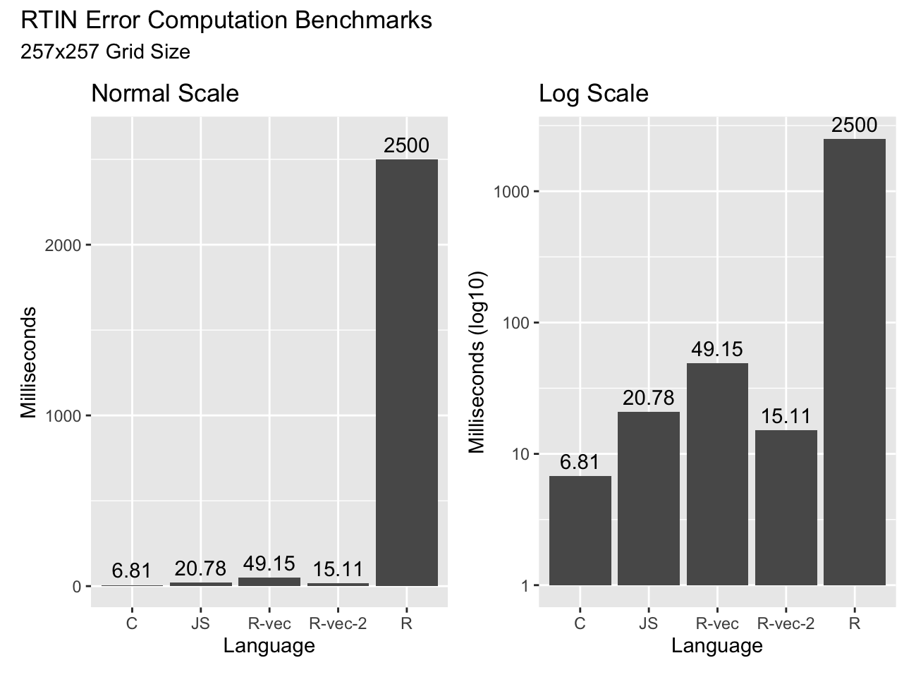
The code as shown (“R-vec”) is about twice as slow as JavaScript, but fifty times faster than the R transliteration of the RTIN algorithm! With some additional optimizations I won’t bore you with (“R-vec-2”) we get to beat out JavaScript. And something remarkable happens as we increase grid sizes:

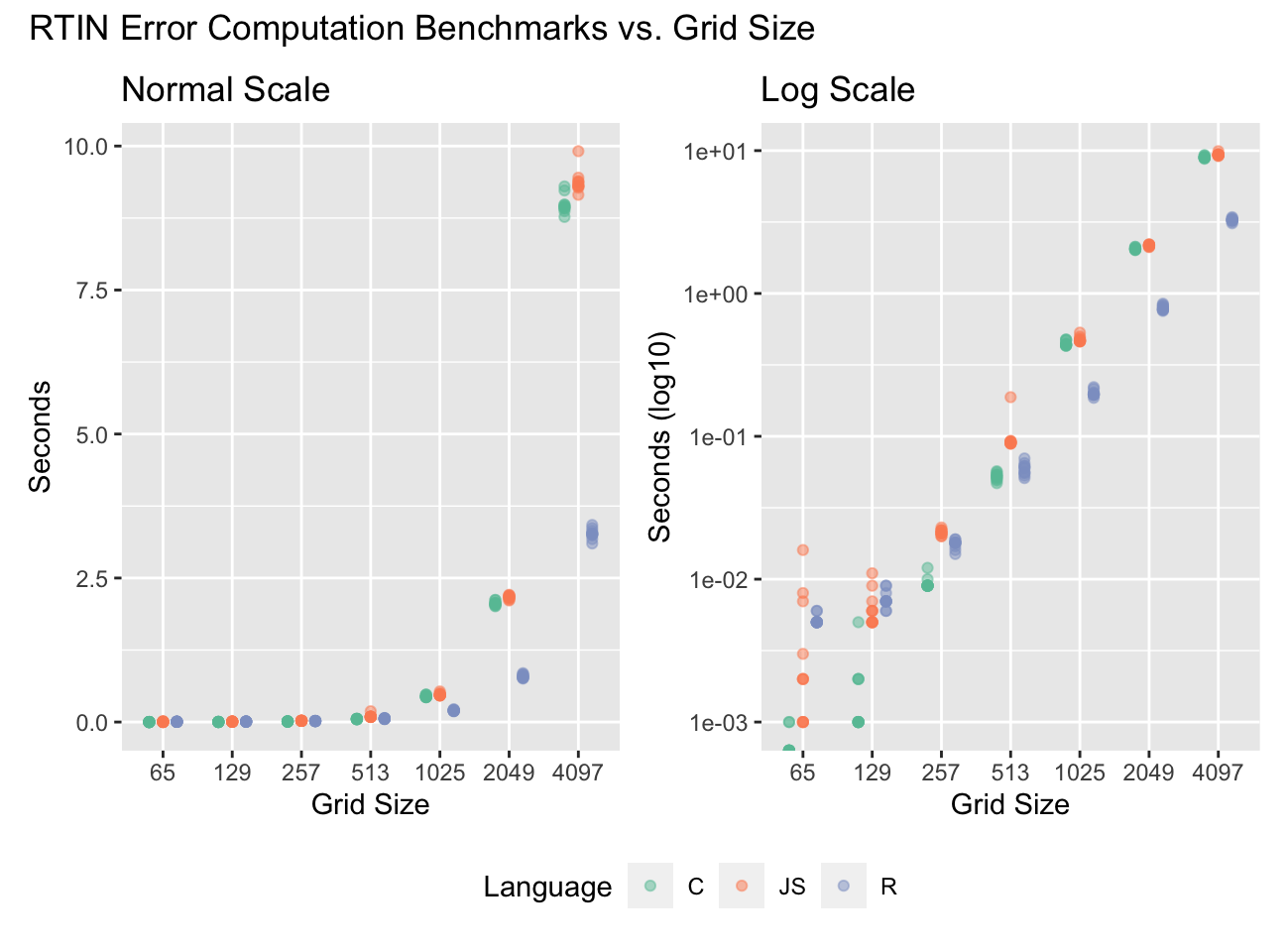
The optimized R implementation (“R-vec-2” from the previous chart) beats both the C and JS implementations by a factor of 2-3x. At the lower sizes the overhead of the R calls holds us back, but as the overall computations increase by $N^2$, the number of R calls only increase by $log(N)$. As the $N^2$ term grows the vectorized algorithm benefits from requiring fewer steps to compute the midpoints.

It is also remarkable that JS does as well as C, perhaps with some more timing volatility due to the overhead of invoking V8 via R and possibly JIT compilation⁹.

Before we move on, a quick recap of some vectorization concepts we applied here:

1. Identify repeating / parallelizable patterns.
2. Structure the data so that the repeating patterns can be processed by internally vectorized¹⁰ functions.
3. Allow R-level loops so long as the number of their iterations is small relative to those carried out in internally vectorized code.

To achieve 2. we resorted to carefully structured seed data, and repeated it either explicitly or implicitly with vector recycling. We did this both for the actual data, as well as for the indices we used to subset the data for use in the vectorized operations.

Too Square

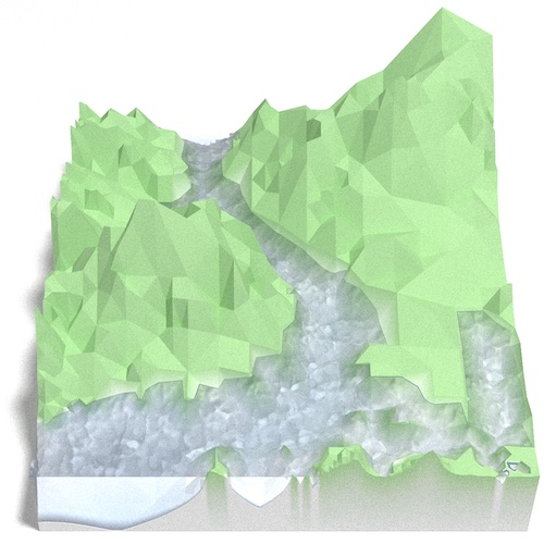
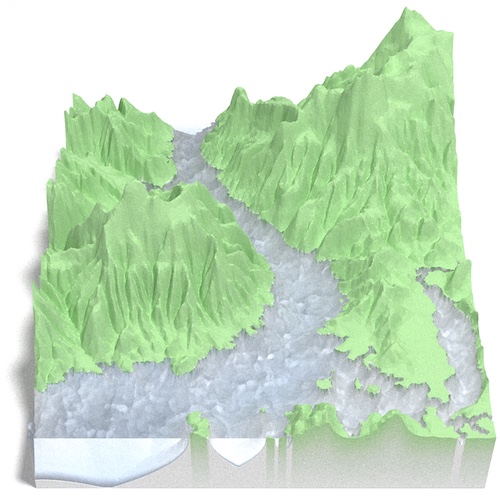
One advantage of directly computing the hypotenuse midpoint coordinates is that we are not limited to $(2^k + 1)$ square elevation maps. With a little extra work we can make the vectorized R implementation support any rectangular map with an odd number of points in both width and height. The “R-vec-2” implementation does exactly that. This allows us to render the 550 x 505 River Derwent DEM by dropping just one row:

The closest dimensions available to the original algorithm are 257 x 257 or 513 x 513, so this is a pretty good feature. A limitation is that the full range of approximation is only available for the $2^k + 1$ grids the original algorithm supports, but there are many useful cases where this doesn’t matter. The best example is stitching together $2^k + 1$ tiles into a larger map that does not conform to $2^k +1$. The most approximate view will be to resolve each tile to two triangles, but there should be no need to go more approximate than that. In exchange you get a larger map with more flexible dimensions that has no inconsistencies at the boundaries, such as this one:

Limits of Vectorization

So far we have completely avoided discussion of the second part of the RTIN algorithm: extraction of approximate meshes subject to an error tolerance. Here an R implementation does worse, but still impressively if we consider that the JavaScript version is JIT compiled into machine code:

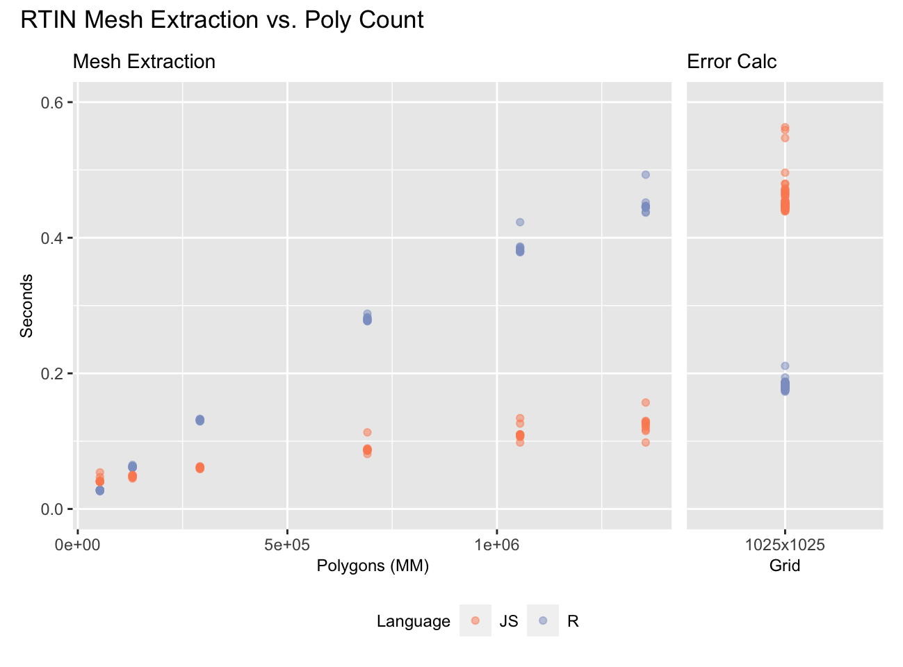
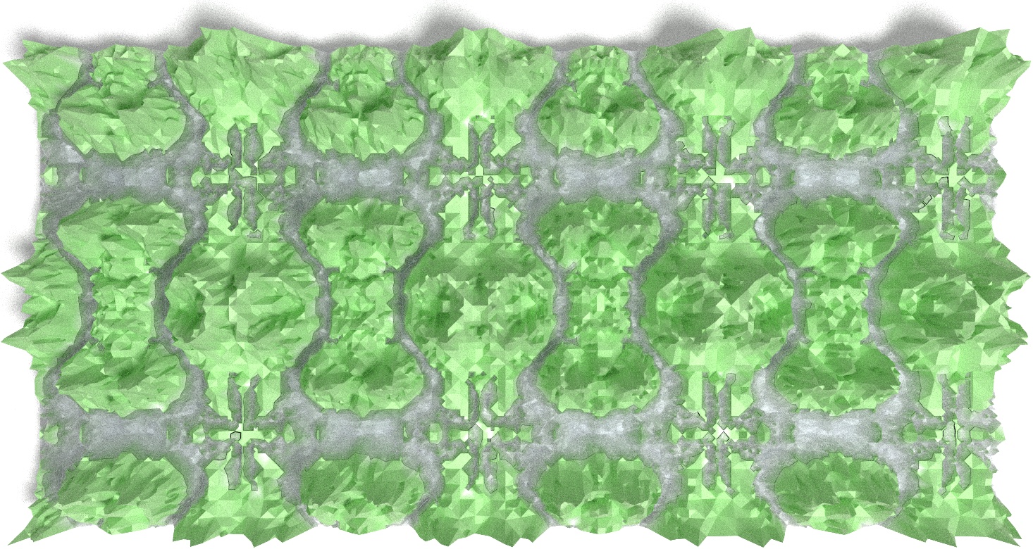
On the 1025 x 1025 grid we tested JS is about as much faster at extracting the meshes (left) as R is at computing the errors (right). How much this matters is a function of how many polygons you extract. The full mesh contains about 2MM polygons, but it looks good with few as ~200K polygons:

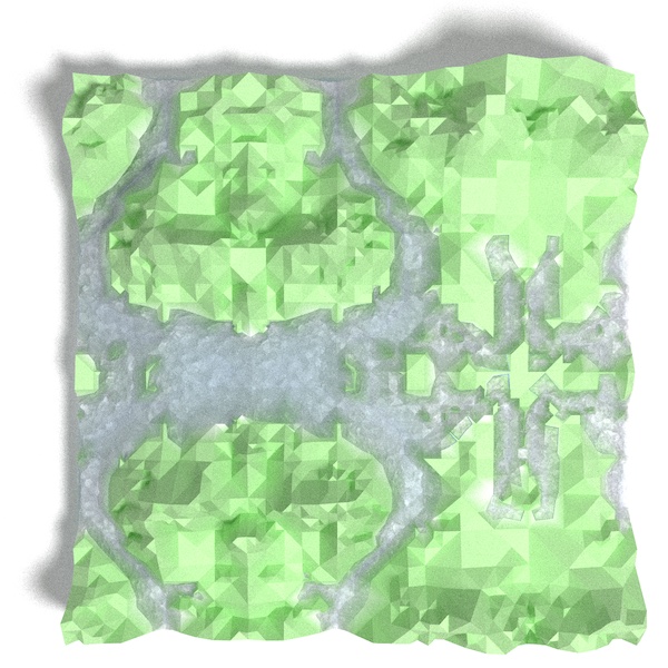
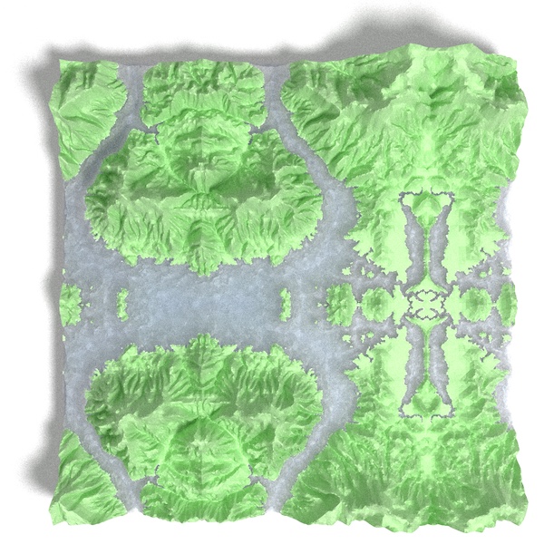
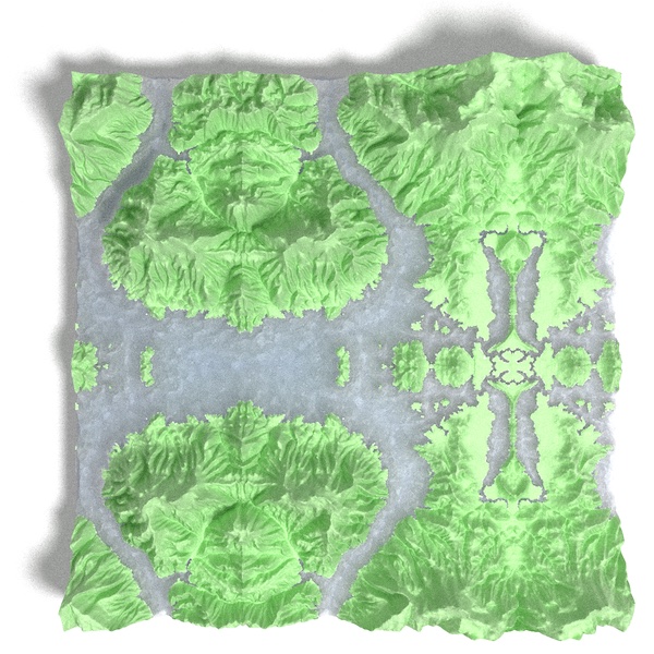
These are all the River Derwent DEM repeated kaleidoscope style to fill 1025 x 1025 maps.

R is able to beat out JavaScript and even C in the error computation because the RTIN algorithm is quite “inefficient”¹¹. Watch it in action again and notice how many steps it takes to compute the location of the first point to compute the error at on a 5 x 5 grid. Compare to how many steps we need with the vectorized algorithm to compute every error on a much larger grid, including child error carry over. I would expect that if we implemented the R version of the algorithm in JavaScript the latter would be faster, assuming the JIT compilation can be as effective as it is with the RTIN algorithm.

Even when algorithms can be fully internally vectorized¹² R is at a disadvantage, usually because vectors need to be re-arranged which requires generating indices and making copies of the vectors. Notwithstanding, for such algorithms it is often possible to get close enough to statically compiled performance that the R implementation is satisfactory.

Conclusions

Despite R being saddled with interpreter overhead, it is often possible to write it in such a way that performance is comparable to statically compiled code. Sometimes it is easy, sometimes it isn’t. Was it worth it in this case? Well, I learned a bit from the process so in the end it was worth it to me. And as a result of this we now have a base-R-only mesh reduction algorithm that works on a much broader set of meshes than the original RTIN.

Appendix

 # Offsets are: parenta, parentb, h midpoint, children with variable number of
 # children supported

offset.dg <- aperm(
  array(
    c(
      0L,0L, 2L,2L, 1L,1L, 1L,2L, 0L,1L, 1L,0L, 2L,1L,
      4L,0L, 2L,2L, 3L,1L, 3L,2L, 4L,1L, 2L,1L, 3L,0L,
      2L,2L, 0L,4L, 1L,3L, 1L,4L, 2L,3L, 0L,3L, 1L,2L,
      2L,2L, 4L,4L, 3L,3L, 3L,4L, 2L,3L, 3L,2L, 4L,3L
    ),
    dim=c(2L, 7L, 4L)
  ),
  c(3L, 1L, 2L)
)
 # Smallest size that allows us to define the children with integer
 # values.
offset.ax <- aperm(
  array(
    c(
      0L,0L, 4L,0L, 2L,0L, 3L,1L, 1L,1L,
      4L,0L, 4L,4L, 4L,2L, 3L,3L, 3L,1L,
      4L,4L, 0L,4L, 2L,4L, 1L,3L, 3L,3L,
      0L,4L, 0L,0L, 0L,2L, 1L,1L, 1L,3L
    ),
    dim=c(2L, 5L, 4L)
  ),
  c(3L, 1L, 2L)
)

init_offsets <- function(i, j, n, layers) {
  axis <- j == 'axis'
  o.raw <- if(axis) offset.ax else offset.dg
  if(!axis && i == layers)
    o.raw <- o.raw[1L,,,drop=F]
  if(axis && i == 1L)
    o.raw <- o.raw[,,1:3,drop=F]

  o.raw <- (o.raw * 2^i) %/% (if(axis) 4L else 2L)
  array(o.raw[,1L,] + o.raw[,2L,] * (n + 1L) + 1L, dim(o.raw)[-2L])
}

compute_error3b <- function(map) {
  n <- nrow(map) - 1
  layers <- log2(n)
  errors <- array(NA_real_, dim=dim(map))

  for(i in seq_len(layers)) {
    for(j in c('axis', 'diag')) {
      ## Initialize template tile
      large.tile <- j == 'diag' && i < layers
      tile.n <- n / 2^(i + large.tile)
      o <- init_offsets(i, j, n, layers)
      o.dim <- dim(o)

      ## Tile rest of surface using template
      seq.r <- (seq_len(tile.n) - 1) * n / tile.n
      o <- rep(o, each=tile.n) + seq.r
      o <- rep(o, each=tile.n) + seq.r * (n + 1)

      ## Identify hypotenuse and its midpoint
      o.i <- seq_len(o.dim[1] * tile.n^2)
      o.len <- length(o.i)
      o.m <- o[o.i + 2 * o.len]
      o.b <- o[o.i + o.len]
      o.a <- o[o.i]

      ## Compute estimate and error at midpoint
      m.est <- (map[o.a] + map[o.b]) / 2
      errors[o.m] <- abs(map[o.m] - m.est)

      ## Retrieve child errors
      err.n <- o.dim[2] - 2
      err.i <- err.vals <- vector('list', err.n)
      for(k in seq_len(err.n)) {
        err.i[[k]] <- o[o.i + o.len * (k + 1)]
        err.vals[[k]] <- errors[err.i[[k]]]
      }
      ## Carry over child errors
      err.val <- do.call(pmax, err.vals)
      err.ord <- order(err.val)
      errors[o.m[err.ord]] <- err.val[err.ord]

      err.i <- NULL
      o <- o.m <- o.a <- o.b <- err.val <- NA
  } }
  errors
}

Session Info

R version 4.0.3 (2020-10-10)
Platform: x86_64-apple-darwin17.0 (64-bit)
Running under: macOS Catalina 10.15.7

Matrix products: default
BLAS:   /Library/Frameworks/R.framework/Versions/4.0/Resources/lib/libRblas.dylib
LAPACK: /Library/Frameworks/R.framework/Versions/4.0/Resources/lib/libRlapack.dylib

locale:
[1] en_US.UTF-8/en_US.UTF-8/en_US.UTF-8/C/en_US.UTF-8/en_US.UTF-8

attached base packages:
[1] stats     graphics  grDevices utils     datasets  methods   base

other attached packages:
[1] inline_0.3.17    patchwork_1.1.0  ambient_1.0.0    rayrender_0.19.0
[5] vetr_0.2.12

loaded via a namespace (and not attached):
 [1] Rcpp_1.0.5       compiler_4.0.3   pillar_1.4.7     later_1.1.0.1
 [5] tools_4.0.3      jsonlite_1.7.1   lifecycle_0.2.0  tibble_3.0.4
 [9] gtable_0.3.0     pkgconfig_2.0.3  rlang_0.4.9      rstudioapi_0.13
[13] yaml_2.2.1       blogdown_0.21    xfun_0.19        dplyr_1.0.2
[17] stringr_1.4.0    roxygen2_7.1.1   xml2_1.3.2       knitr_1.30
[21] generics_0.1.0   vctrs_0.3.5      tidyselect_1.1.0 grid_4.0.3
[25] glue_1.4.2       R6_2.5.0         processx_3.4.5   bookdown_0.21
[29] ggplot2_3.3.2    purrr_0.3.4      magrittr_2.0.1   servr_0.20
[33] scales_1.1.1     ps_1.4.0         promises_1.1.1   ellipsis_0.3.1
[37] colorspace_2.0-0 httpuv_1.5.4     stringi_1.5.3    munsell_0.5.0
[41] crayon_1.3.4

This is an HTML Canvas flipbook that displays key frames of an animation in a more controllable manner than in a video player. If you are reading this text your browser does not support HTML Canvas.

    FPS:   #: /   ⤾: