Off Course, of Course

A few months ago I stumbled on Vladimir Agafonkin’s (@mourner) fantastic observable notebook on adapting the Will Evans etal. Right-Triangulated Irregular Networks (RTIN) algorithm to JavaScript. The subject matter is interesting and the exposition superb. I’ll admit I envy the elegance of natively interactive notebooks.

I almost left it at that, but then the irrepressible “can we do that in R” bug bit me. I might be one of the few folks out there actually afflicted by this bug, but that’s neither here nor there. It doesn’t help that this problem also presents some interesting visualization challenges, so of course I veered hopelessly off-course¹ and wrote this post about it.

Why write a post about visualizing MARTINI when @mourner already does it in his? Well, we’re trying to reformulate the algorithm for efficient use in R, and the MARTINI post focuses mostly on what the algorithm does, a little bit on why it does it, and not so much on how it does it. So this post will focus on the last two. Besides, I’m looking for an excuse to rayrender stuff.

Why reformulate a perfectly fine JS algorithm into R, particularly when we could just trivially port it to C and interface that into R? Or even just run it in R via R V8? For the sport of it, duh.

Right Triangles

The RTIN algorithm generates triangle meshes that approximate surfaces with elevations defined on a regular grid in the x-y plane. The beloved volcano height map that comes bundled with R is exactly this type of surface. Approximations can be constrained to an error tolerance, and here we show the effect of specifying those tolerance on volcano as a percentage of its total height:

We’re not going to evaluate the effectiveness of this method at generating approximation meshes as our focus is on the mechanics of the algorithm. That said, it’s noteworthy that the “2%” approximation reduces the polygon count over five-fold and looks good even absent shading tricks.

One of the things that pulled me into this problem is the desire to better visualize the relationship between the original mesh and its various approximations. This is easily solved with lines in 2D space with superimposition, but becomes more difficult with 2D surfaces in 3D space. Occlusion and other artifacts from projection of the surfaces onto 2D displays get in the way. Possible solutions include juxtaposing in time as in @mourner’s notebook with the slider, or faceting the 2D space as I did above, but neither lets us see the details of the differences.

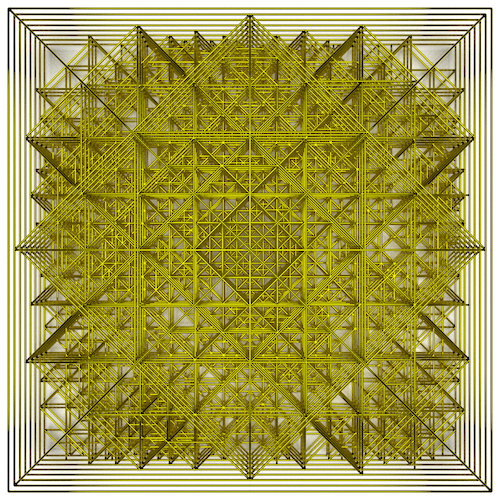
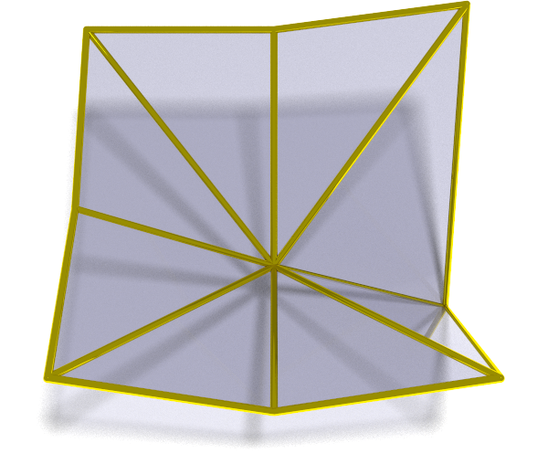
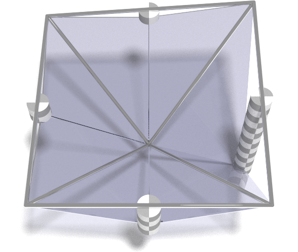
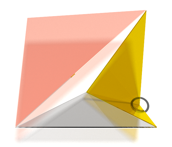
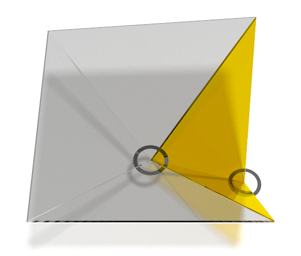
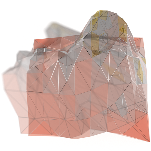
I ended up settling on the “à-la-Pyramide-du-Louvre” style visualization:

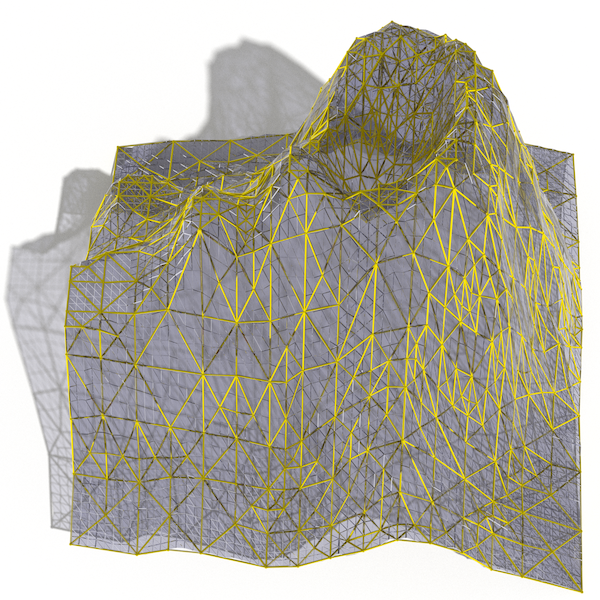
Look closely (do zoom in!) particularly at the coarser approximations, and you will see where the surface weaves in and out of the approximations. You might even notice that all the vertices of the approximation coincide with surface vertices. This is because the approximated meshes are made from subsets of the vertices of the original surface.

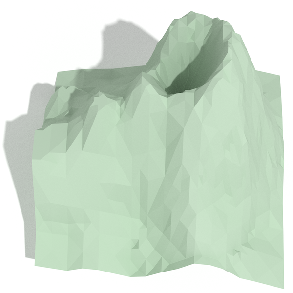
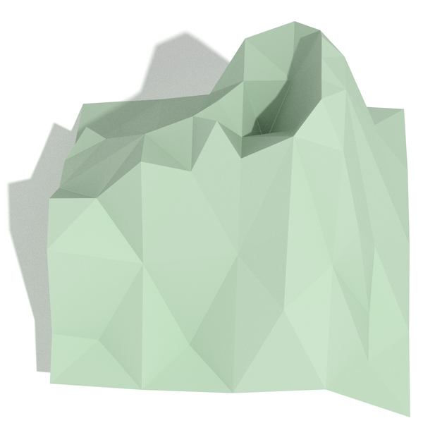
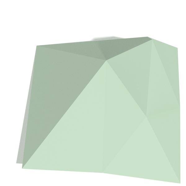
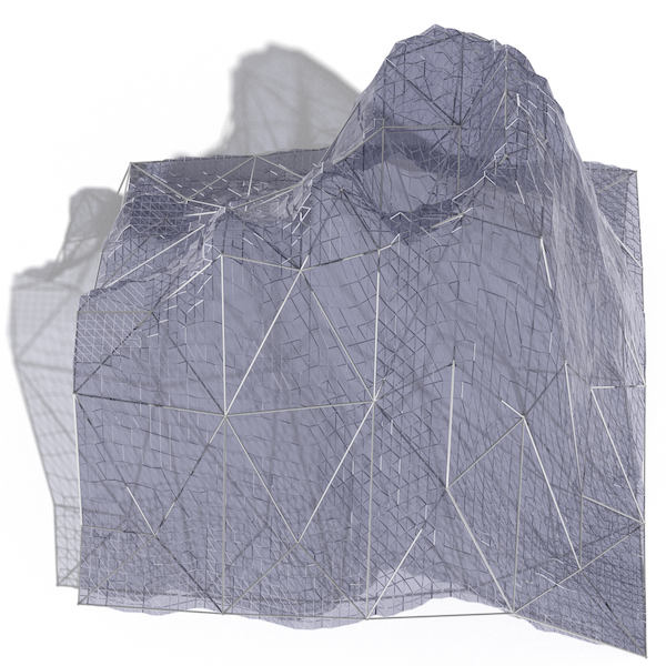
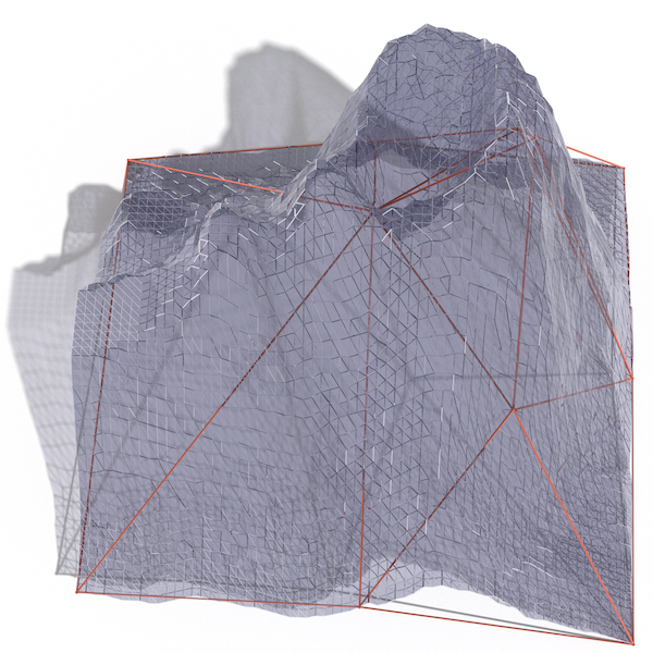
Unfortunately even when realistically ray traced, 3D images projected onto 2D inevitably lose… depth. We can compensate by presenting different perspectives so that our brains use the parallax for additional depth perception. Sorry volcano, but I only do this to you about once a year, and it’s always for a good cause.

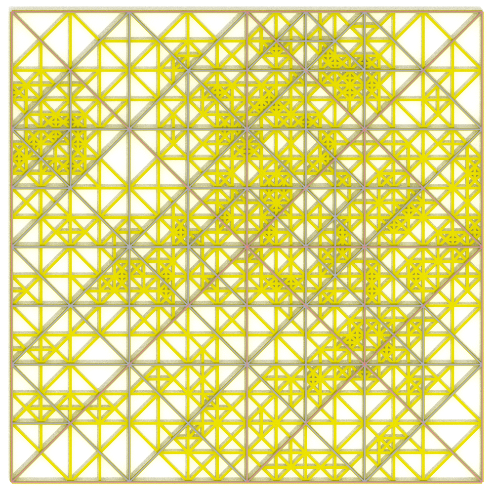
Let’s flatten the elevation component of the meshes to look at their 2D structure:

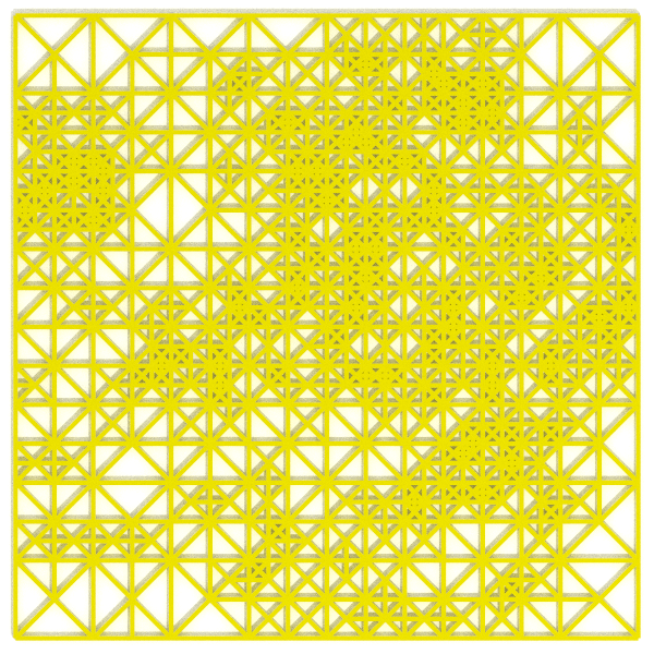
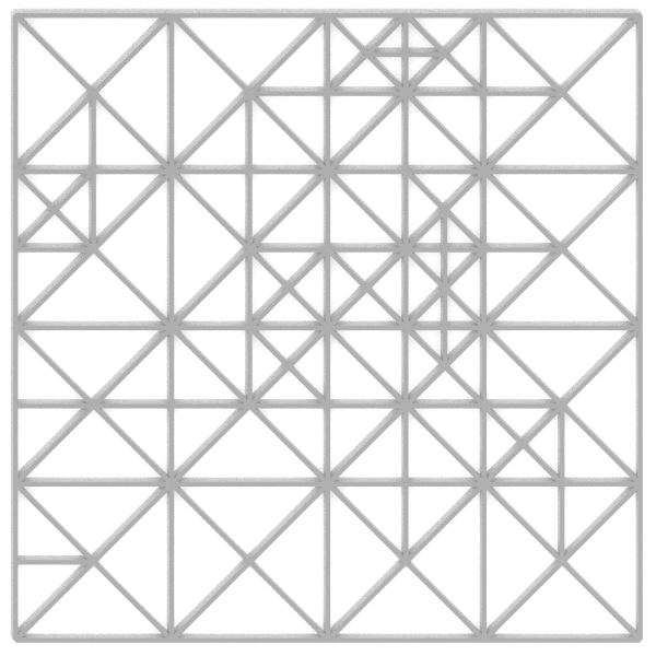
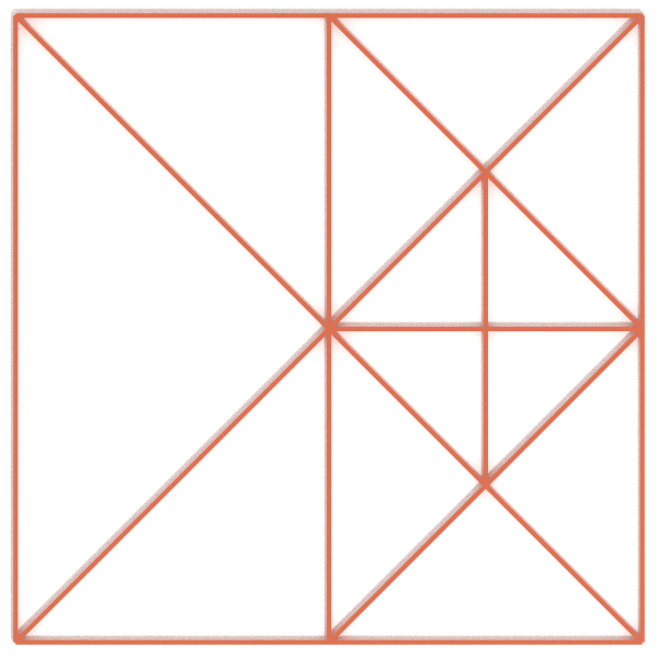
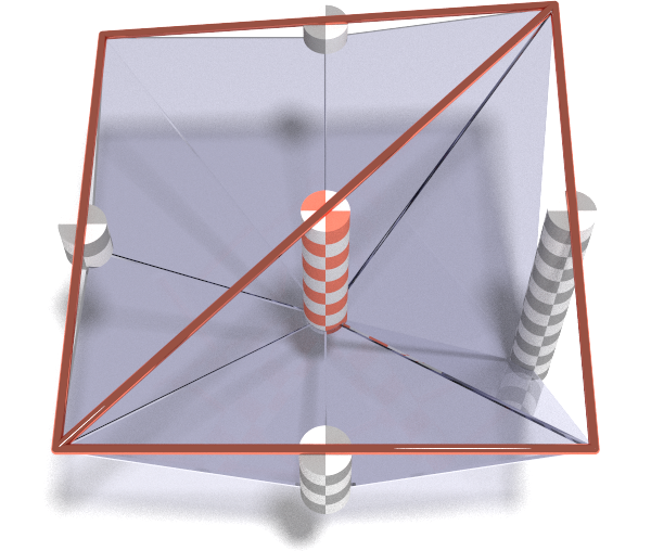
In the x-y plane all the triangles are right angled isoceles triangles. This is where the “Right-Triangulated” part of the algorithm name comes from. Another important feature of this mesh approximation is that it is hierarchical. When we stack the three meshes we can see that each of the larger triangles in the low fidelity meshes is exactly replaced by a set of triangles from the higher fidelity ones:

If you look closely you’ll see that edges of larger triangles never cross the faces of the smaller ones. This is because the smaller triangles are made by adding a vertex in the middle of the long edge of a larger triangle and connecting it to the opposite vertex. Every edge of the larger triangle overlaps with an edge of the smaller triangles. As we’ll see in the next post this creates an important constraint on how the different approximation layers are calculated.

Errors

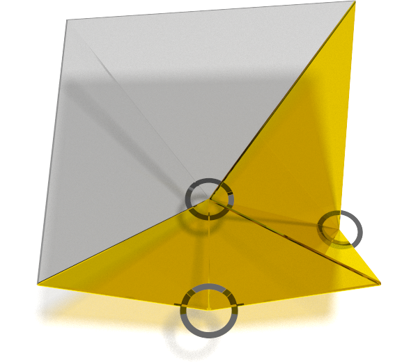
We’ve seen that MARTINI allows us to extract approximation meshes subject to a particular error tolerance. At some point we have to calculate the approximation error we test against the tolerance. We’ll illustrate this with a minimal 3x3 elevation the sake of clarity:

At the most granular level (gold) there is no error as the mesh corresponds exactly to the elevation surface. Recall that the smaller triangles are made by splitting larger triangles in the middle of their long edge. At the first level of approximation (silver) those are the midpoints of the peripheral edges. We show the errors at those locations with the grey checked cylinders. At the next level of approximation (copper) we repeat the process. This time the long edge runs across the middle of the mesh so the error is measured dead center.

An implication of measuring error at the point we combine the smaller triangles into bigger ones is that we never measure errors from different levels of approximation at overlapping locations. As such we can store the errors in a matrix the same size as the surface, whether a simple 3 x 3 surface or a more complex one like volcano²:

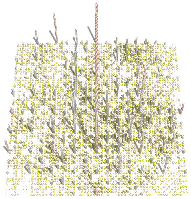
The above matrices contain the errors for every level of approximation. We only need to calculate the matrix once, and thereafter we can test it against different tolerance thresholds to determine what approximation mesh to draw.

Surface Extraction

We will play through the process of extracting meshes at different tolerance levels. The idea is the extract the coarsest mesh without any errors above the threshold. Resolving errors is easy: just break a triangle long edge such that a vertex is added at any of the surface points for which the error is too high. That vertex will be on the original surface and as such have no error.

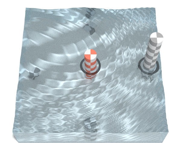
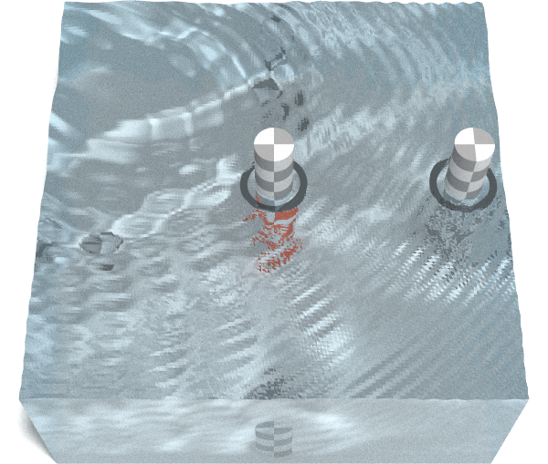
Let’s illustrate the process with our 3x3 error matrix, and our error tolerance represented as a “water” level. Errors peeking above the surface exceed the tolerance and must be addressed:

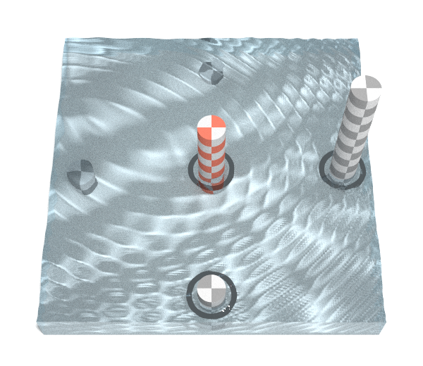
For each of the three errors that exceed our threshold we split the corresponding triangle in the middle of the long edge. This causes us to break up the bottom-right part of the surface into the highest detail triangles (gold), but lets us use the first level of approximation for the top left (grey).

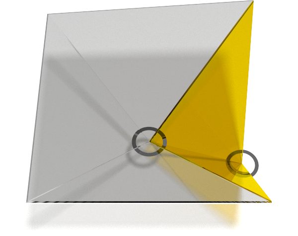
As we increase our tolerance we can extend the approximation to the bottom of the surface:

But if we further increase our tolerance we run into problems:

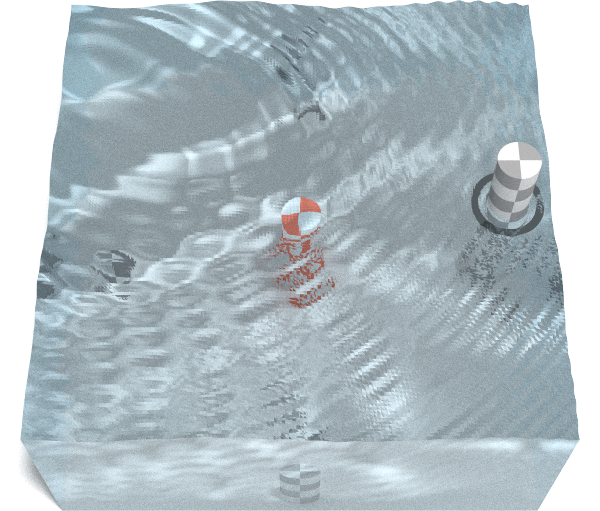
Breaking the right-most triangle led us to break the containing triangle (bottom-right half) even though error in the middle of the surface is below our threshold. Anytime we split a triangle, all the ancestor triangles that contain it will need to be split as well. But that is not sufficient as demonstrated by the remaining gap in the mesh. We must also break up any ancestor siblings that share an edge with the edges that are split.

You can imagine how this might complicate our mesh extraction. We need to check a point’s error, but also the errors of any of its children, and the children of its siblings.

One clever solution to this is to ensure that the error at any given point is the greater of the actual error, or the errors associated with its children. Then, if we compute error from smallest triangles to larger ones, we can carry over child errors to the parents:

In this case we carry over the error from the right child from the first level of approximation onto the second level. We actually carry over the error from all four next-generation vertices, it just so happens in this case there is only one that has an error greater than the parent. With this logic our mesh extraction can work correctly without any additional logic:

Algorithm in Action

We now have a rough idea of the algorithm. Unfortunately I learned the hard way that “a rough idea” is about as useful when refactoring an algorithm as it is to know that a jar of nitroglycerin is “kinda dangerous” when you’re tasked with transporting it. In order to safely adapt the algorithm to R we need full mastery of the details. Well at least I for one would have more hair left on my head if I’d achieved some level of mastery instead of just trying to wing it.

We will focus on the error computation over the mesh extraction algorithm as that is the more complicated part of the process. Its outline follows:

for (every triangle in mesh) {
  while (searching for target triangle coordinates) {
    # ... Compute coordinates of vertices `a`, `b`, and `c` ...
  }
  # ... Compute approximation error at midpoint of `a` and `b` ...
}

The for loop iterates as many times as there are triangles in the mesh. In our 3 x 3 grid there are six triangles (4 at the first level of approximation, and another 2 at the next level). In reality there are another eight triangles at the most detailed level, but the algorithm ignores those by definition they have no error. For each of the checked triangles, the while loop identifies their vertex coordinates $(ax,ay)$, $(bx,by)$, and $(cx,cy)$, which we can use to compute the error at the middle of the long edge, and as a result the approximation error.

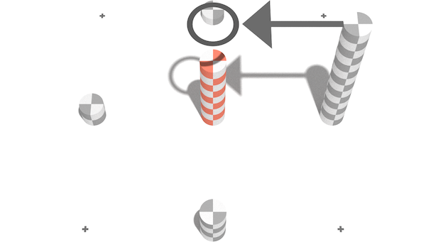
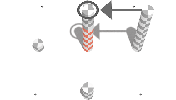
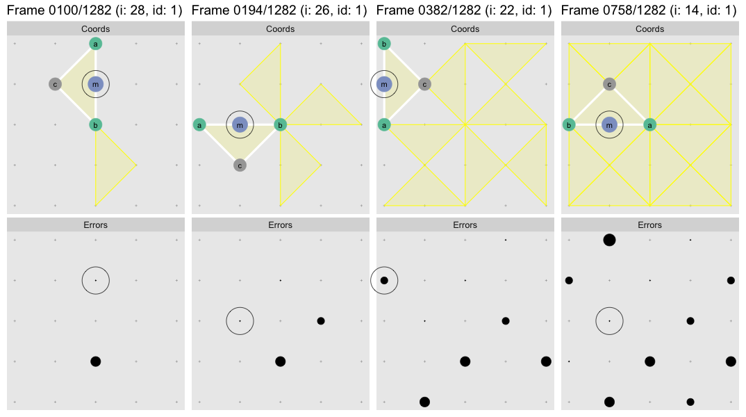
Let’s observe the algorithm in action, but we’ll use a 5 x 5 grid this time³. Regrettably we’ll abandon the 3D realm for the sake of clarity. In this flipbook we watch the algorithm find the first triangle to get a sense for how it works. The visualization is generated with the help of watcher. Each frame displays the state of the system after the evaluation of the highlighted line:

When the while loop ends the first target triangle has been found, shown in yellow. In the subsequent frames the algorithm computes the location of the midpoint m of the points a and b (these two always define to the long edge), computes the approximation error at that point, and in the last frame records it to the error matrix. Since we’re stuck in 2D we now use point size rather than cylinder height to represent error magnitude.

You can click/shift-click on the flipbook to step forward/back to see clearly what each step of the algorithm is doing. We stopped the flipbook before the child error propagation step as at the first level there are no child errors to propagate⁴.

What happens next is pretty remarkable. At the top of the loop we’re about to repeat we have:

for (i in (nTriangles - 1):0) {
  id <- i + 2L
  # ... rest of code omitted

This innocent-seeming reset of id will ensure that the rest of the logic finds the next smallest triangle, and the next after that, and so forth:

At this point we’ve tiled the whole surface at the most granular approximation level, but we need to repeat the process for the next approximation level. Remarkably the smaller initial id values cause the while loop to exit earlier at the next larger triangle size. Here is another flipbook showing the search for the second triangle of the next approximation level⁵:

The last few frames show how the error from the children elements (labeled lc and rc for “left child” and “right child”) carry over into the current target point. As we saw earlier this ensures there are no gaps in our final mesh. Each error point will have errors carried over from up to four neighboring children. For the above point the error from the remaining children is carried over a few hundred steps later when the adjoining triangle is processed:

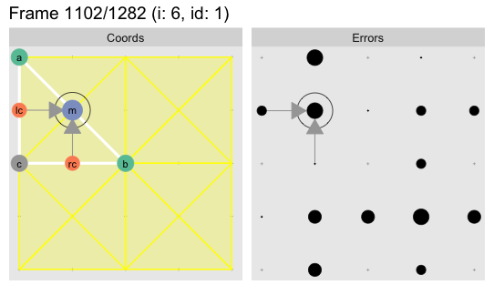
In this case it the additional child errors are smaller so they do not change the outcome, but it is worth noting that each long edge midpoint may have up to four child errors added to it.

Here is the whole thing at 60fps:

R’s Kryptonite

For the algorithm visualization we “transliterated”⁶ the JavaScript algorithm into R. While this works, it does so slowly. Compare the timings of our R function, the JavaScript version, and finally a C version:

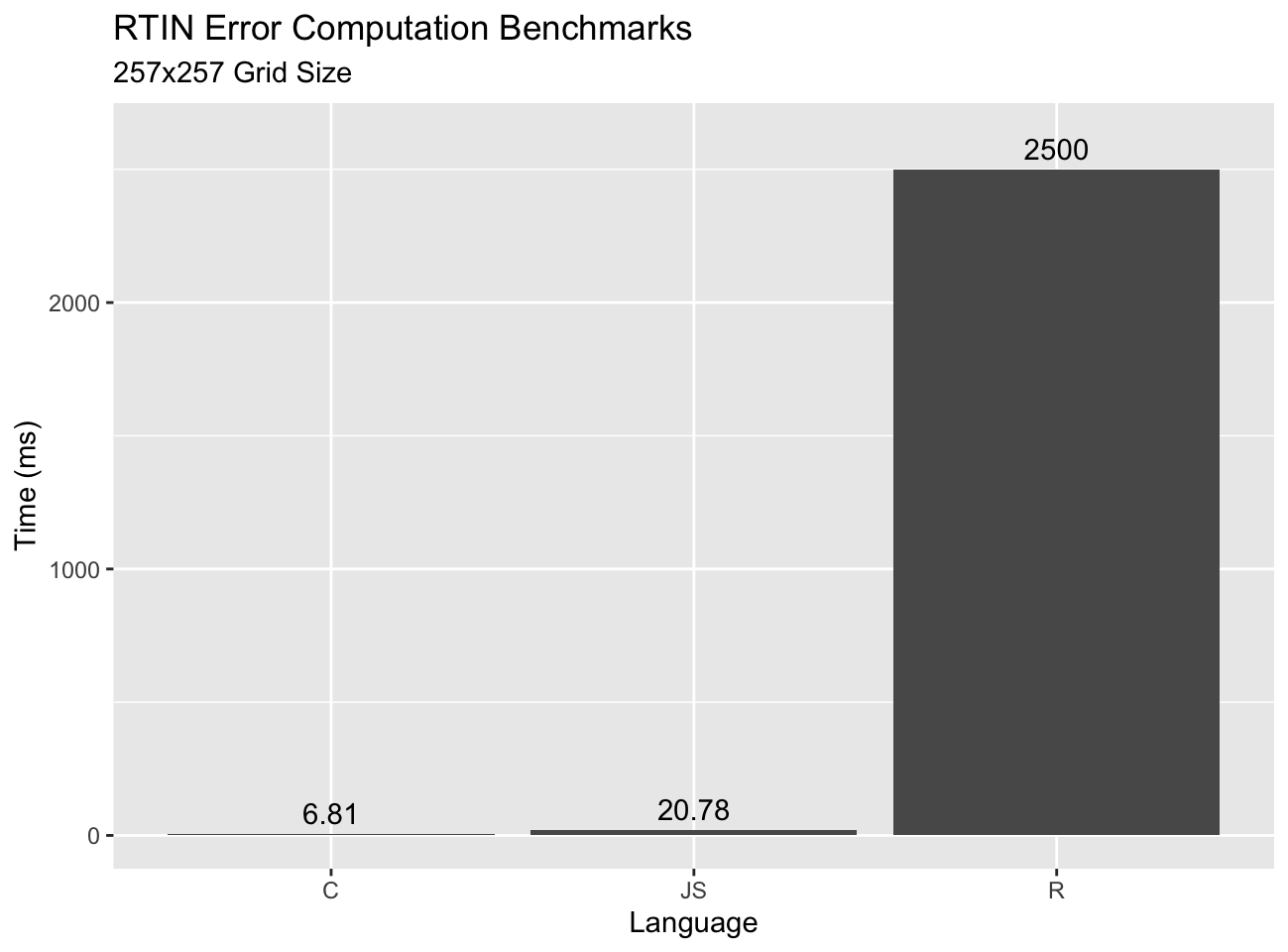
I was surprised by how well JS stacks up relative to C. Certainly a ~3x gap is nothing to sneeze at, but I expected it to be bigger given JS is interpreted⁷. On the other hand R does terribly. This is expected as R is not designed to run tight loops on scalar values. We could take some steps to get the loop to run a little faster, but not to run fast enough to run in real-time at scale.

Let’s Vectorize the Absolute $#!+ Out Of This

So what are we #rstats users to do? Well, as @mdsumner enthusiastically puts it:

JavaScript is cool, C++ is cool. But #rstats can vectorize the absolute shit out of this. No loops until triangle realization

– @mdsumner

Indeed, we don’t need to watch the algorithm play out very long to see that its elegance comes at the expense of computation. Finding each triangle requires many steps. It should be possible to compute each triangle’s coordinates directly and independently of the others, which means we should be able to vectorize the process.

So, let’s go vectorize the absolute $#!+ out of this. It’ll be fun! If you’re into that type of thing anyway. Stay tuned for RTINI Part II.

Appendix

errors_rtin2

function(terrain) {
  errors <- array(NA_real_, dim(terrain))
  nSmallestTriangles <- prod(dim(terrain) - 1L)
  nTriangles <- nSmallestTriangles * 2 - 2
  lastLevelIndex <-
    nTriangles - nSmallestTriangles
  gridSize <- nrow(terrain)
  tileSize <- gridSize - 1L

  # Iterate over all possible triangles,
  for (i in (nTriangles - 1):0) {
    id <- i + 2L
    mx <- my <- rcx <- rcy <- lcx <- lcy <-
      ax <- ay <- bx <- by <- cx <- cy <- NA
    if (bitwAnd(id, 1L)) {
      # Bottom-right triangle
      bx <- by <- cx <- tileSize
      ax <- ay <- cy <- 0
    } else {
      # Top-left triangle
      ax <- ay <- cy <- tileSize
      bx <- by <- cx <- 0
    }
    # Find target triangle
    while ((id <- (id %/% 2)) > 1L) {
      tmpx <- (ax + bx) / 2
      tmpy <- (ay + by) / 2

      if (bitwAnd(id, 1L)) {
        # Right sub-triangle
        bx <- ax
        by <- ay
        ax <- cx
        ay <- cy
      } else {
        # Left sub-triangle
        ax <- bx
        ay <- by
        bx <- cx
        by <- cy
      }
      cx <- tmpx
      cy <- tmpy
    }
    az <- terrain[ax + 1, ay + 1]
    bz <- terrain[bx + 1, by + 1]
    interpolatedHeight <- (az + bz) / 2

    # Error at hypotenuse midpoint
    mx <- ((ax + bx) / 2)
    my <- ((ay + by) / 2)
    mz <- terrain[mx + 1, my + 1]
    middleError <- max(na.rm=TRUE,
      abs(interpolatedHeight - mz),
      errors[mx+1, my+1]
    )
    errors[mx+1, my+1] <- middleError

    # Propagate child errors
    lcError <- rcError <- 0
    if (i < lastLevelIndex) {
      lcx <- (ax + cx) / 2
      lcy <- (ay + cy) / 2
      lcError <- errors[lcx+1, lcy+1]
      rcx <- (bx + cx) / 2
      rcy <- (by + cy) / 2
      rcError <- errors[rcx+1, rcy+1]
    }
    errors[mx+1, my+1] <- max(
      errors[mx+1, my+1], lcError, rcError
    )
  }
  # Clear and exit
  mx <- my <- rcx <- rcy <- lcx <- lcy <-
    ax <- ay <- bx <- by <- cx <- cy <- NA
  errors
}

errors_rtin_c <- inline::cfunction(sig=c(terr='numeric', grid='integer'), body="
  int gridSize = asInteger(grid);
  int tileSize = gridSize - 1;
  SEXP errSxp = PROTECT(allocVector(REALSXP, gridSize * gridSize));
  double * terrain = REAL(terr);
  double * errors = REAL(errSxp);
  errors[0] = errors[gridSize - 1] = errors[gridSize * gridSize - 1] =
    errors[gridSize * gridSize - gridSize] = 0;

  int numSmallestTriangles = tileSize * tileSize;
  // 2 + 4 + 8 + ... 2^k = 2 * 2^k - 2
  int numTriangles = numSmallestTriangles * 2 - 2;
  int lastLevelIndex = numTriangles - numSmallestTriangles;

  // iterate over all possible triangles, starting from the smallest level
  for (int i = numTriangles - 1; i >= 0; i--) {

    // get triangle coordinates from its index in an implicit binary tree
    int id = i + 2;
    int ax = 0, ay = 0, bx = 0, by = 0, cx = 0, cy = 0;
    if (id & 1) {
      bx = by = cx = tileSize; // bottom-left triangle
    } else {
      ax = ay = cy = tileSize; // top-right triangle
    }
    while ((id >>= 1) > 1) {
      int mx = (ax + bx) >> 1;
      int my = (ay + by) >> 1;

      if (id & 1) { // left half
        bx = ax; by = ay;
        ax = cx; ay = cy;
      } else { // right half
        ax = bx; ay = by;
        bx = cx; by = cy;
      }
      cx = mx; cy = my;
    }
    // calculate error in the middle of the long edge of the triangle
    double interpolatedHeight =
      (terrain[ay * gridSize + ax] + terrain[by * gridSize + bx]) / 2;
    int middleIndex = ((ay + by) >> 1) * gridSize + ((ax + bx) >> 1);
    double middleError = abs(interpolatedHeight - terrain[middleIndex]);

    if (i >= lastLevelIndex) { // smallest triangles
      errors[middleIndex] = middleError;

    } else { // bigger triangles; accumulate error with children
      double leftChildError =
        errors[((ay + cy) >> 1) * gridSize + ((ax + cx) >> 1)];
      double rightChildError =
        errors[((by + cy) >> 1) * gridSize + ((bx + cx) >> 1)];

      double tmp = errors[middleIndex];
      tmp = tmp > middleError ? tmp : middleError;
      tmp = tmp > leftChildError ? tmp : leftChildError;
      tmp = tmp > rightChildError ? tmp : rightChildError;
      errors[middleIndex] = tmp;
    }
  }
  UNPROTECT(1);
  return errSxp;
")

System Info

This is an HTML Canvas flipbook that displays key frames of an animation in a more controllable manner than in a video player. If you are reading this text your browser does not support HTML Canvas.

    FPS:   #: /   ⤾: