If Only We Could See Code In Action

I recently got caught up trying to port a JavaScript algorithm¹ into R. A direct port would have been straightforward (and slow), but I wanted to vectorize it. I had a rough idea what the algorithm did from the description and from the code, but because I did not understand the semantics exactly I wasted a lot of time on bad implementations. It wasn’t until I buckled up and figured out how to step through the JS version in my browser console and painstakingly recorded what was happening that I finally got things right.

Even though I resolved the issue the experience left me wanting for a better way of visualizing algorithms in action.

Instrumenting R Functions

One of R’s lesser known super-powers is its ability to manipulate unevaluated R code. We used this to instrument an R RPN parser, which in turn allowed us to visualize it in action. Unfortunately the instrumentation was specific to that function, and generalizing it for use with the R translation of the JS algorithm felt like too much work.

How does instrumentation work? The basic concept is to modify each top-level statement to trigger a side effect. For example if we start with:

f0 <- function() {
  1 + 1
}
f0()

[1] 2

With some language manipulation we can get:

f1 <- function() {
  {
    message("I'm a side effect")
    1 + 1
  }
}
f1()

I'm a side effect

[1] 2

The functions produce the same result, but the second one triggers a side effect. In this case the side effect is to issue a message, but we could have instead recorded variable values. In other words, the side effect is the instrumentation. I first saw this concept in Jim Hester’s wonderful covr package where it is used to measure test code coverage.

Of course only after my need for a generalized instrumentation tool passed, I got the irrepressible urge to write one. So I quickly threw something together into the watcher package. It’s experimental, limited², but does just enough for my purposes.

watcher ships with an implementation of the insertion sort algorithm for demonstration purposes:

library(watcher) # you'll need to install from github for this
insert_sort

function (x) 
{
    i <- 2
    while (i <= length(x)) {
        j <- i
        while (j > 1 && x[j - 1] > x[j]) {
            j <- j - 1
            x[j + 0:1] <- x[j + 1:0]
        }
        i <- i + 1
    }
    x
}
<bytecode: 0x7f8d1160f070>
<environment: namespace:watcher>

We can use watcher::watch to transmogrify insert_sort into its instrumented cousin insert_sort_w:

insert_sort_w <- watch(insert_sort, c('i', 'j', 'x'))

This new function works exactly like the original, except that the values of the specified variables are recorded at each evaluation step and attached to the result as an attribute:

set.seed(1220)
x <- runif(10)
x

 [1] 0.0979 0.2324 0.0297 0.3333 0.5672 0.4846 0.4145 0.6775 0.3080 0.5123

insert_sort(x)

 [1] 0.0297 0.0979 0.2324 0.3080 0.3333 0.4145 0.4846 0.5123 0.5672 0.6775

all.equal(insert_sort(x), insert_sort_w(x), check.attributes=FALSE)

[1] TRUE

We can retrieve the recorded data from the “watch.data” attribute:

dat <- attr(insert_sort_w(x), 'watch.data')
str(dat[1:2])  # show first two steps

List of 2
 $ :List of 2
  ..$ i: num 2
  ..$ x: num [1:10] 0.0979 0.2324 0.0297 0.3333 0.5672 ...
  ..- attr(*, "line")= int 3
 $ :List of 2
  ..$ i: num 2
  ..$ x: num [1:10] 0.0979 0.2324 0.0297 0.3333 0.5672 ...
  ..- attr(*, "line")= int 4

watcher::simplify_data combines values across steps into more accessible structures. For example, scalars are turned into vectors with one element per step:

dat.s <- simplify_data(dat)
head(dat.s[['.scalar']])

  .id .line i  j
1   1     3 2 NA
2   2     4 2 NA
3   3     5 2  2
4   4     6 2  2
5   5    10 3  2
6   6     4 3  2

.id represents the evaluation step, and .line the corresponding line number from the function.

Visualizing Algorithms

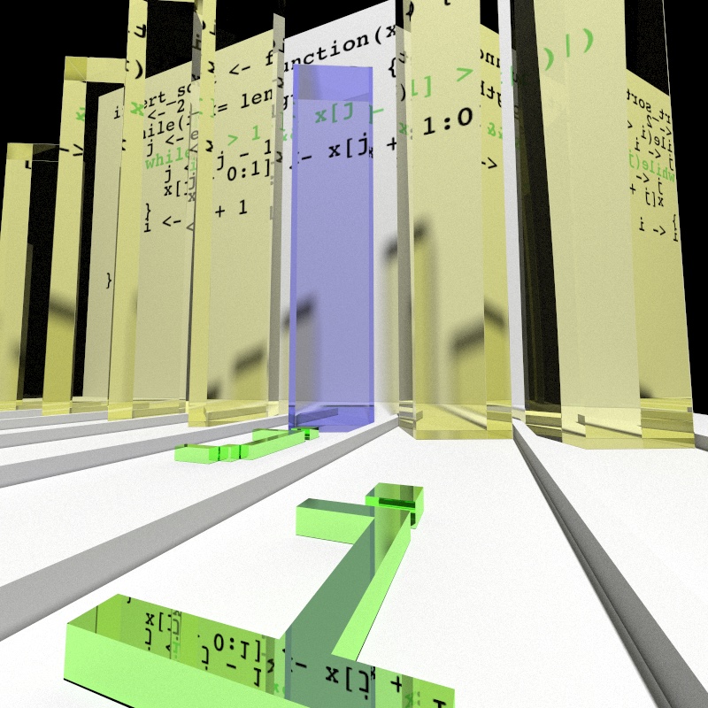
watcher provides all the data we need to visualize the algorithm, but unfortunately that is as far as it goes. Actual visualization requires a human to map values to aesthetics. For example, here we render the values of x as the height of 3D glass bars. Certainly we all know that 3D bar charts are bad, but 3D bar charts made of ray-traced dielectrics? Surely there can be nothing better!

If you would rather mine bitcoin³ with your CPU cycles we can settle for a 2D flipbook. From a pedagogical standpoint this is probably a more effective visualization, if a bit flat in comparison:

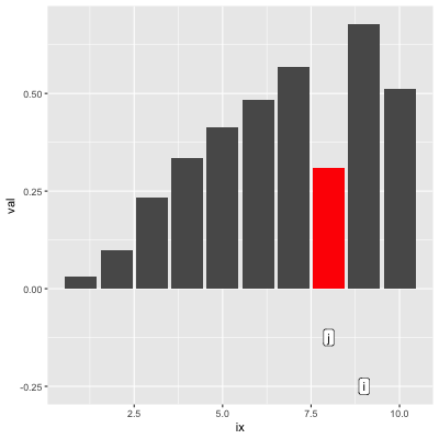
If we’re content with just the right hand side of the boring 2D visualization it is pretty easy to create that:

# Extract x data and augment with the corresponding scalar `j` loop index

xs <- dat.s[['x']]
xs <- transform(
  xs, j=dat.s[['.scalar']][['j']][.id], ix=rep_len(seq_along(x), length(val))
)
# Data for labels

labs <- reshape2::melt(dat.s[['.scalar']][c('.id', 'i', 'j')], id.var='.id')

# Plot!

library(ggplot2)
p <- ggplot(xs, aes(x=ix, y=val)) +
  geom_col(aes(fill=I(ifelse(!is.na(j) & ix==j, 'red', 'grey35')))) +
  geom_label(
    data=labs, aes(x=value, label=variable, y=-0.25 + (variable=='j') * .125)
  ) +
  gganimate::transition_manual(.id)

This will produce an approximation of the right hand side of the flipbook (showing frame 50 here):

But things get tricky beyond that. Juxtaposing the code is challenging and would benefit from some tools to render the text and graphics independently. My own ggplot implementation requires horrid text positioning hacks.

Transitioning to the ray-traced version was relatively easy⁴ thanks to the surprisingly full-featured and all-around awesome rayrender package by Tyler Morgan Wall. I did have to deploy my rendering farm⁵ though.

Conclusions

I’m unsure if watcher does enough to make visualizing algorithms more generally practical. Perhaps automated handling of the code rendering and juxtaposition would make this easy enough to be worth the trouble. On the flipside, as algorithms become more complex figuring out aesthetic mappings that intuitively represent them becomes increasingly difficult. Finally, while R provides some great tools for instrumenting and visualizing algorithms, the static nature of the output limits the possibilities for interactive visualizations.

Appendix

template <- call('{', quote(message("I'm a side effect")), NULL)
template

{
    message("I'm a side effect")
    NULL
}

f1 <- f0
template[[3]] <- body(f1)[[2]]
body(f1)[[2]] <- template
f1

function () 
{
    {
        message("I'm a side effect")
        1 + 1
    }
}

insert_sort_w

function (x) 
{
    watcher:::watch_init(c("i", "j", "x"))
    res <- {
        {
            .res <- (i <- 2)
            watcher:::capture_data(environment(), 3L)
            .res
        }
        while ({
            .res <- (i <= length(x))
            watcher:::capture_data(environment(), 4L)
            .res
        }) {
            {
                .res <- (j <- i)
                watcher:::capture_data(environment(), 5L)
                .res
            }
            while ({
                .res <- (j > 1 && x[j - 1] > x[j])
                watcher:::capture_data(environment(), 6L)
                .res
            }) {
                {
                  .res <- (j <- j - 1)
                  watcher:::capture_data(environment(), 7L)
                  .res
                }
                {
                  .res <- (x[j + 0:1] <- x[j + 1:0])
                  watcher:::capture_data(environment(), 8L)
                  .res
                }
            }
            {
                .res <- (i <- i + 1)
                watcher:::capture_data(environment(), 10L)
                .res
            }
        }
        {
            .res <- (x)
            watcher:::capture_data(environment(), 12L)
            .res
        }
    }
    attr(res, "watch.data") <- watcher:::watch_data()
    attr(res, "watch.code") <- c("insert_sort <- function (x) ", 
    "{", "    i <- 2", "    while (i <= length(x)) {", "        j <- i", 
    "        while (j > 1 && x[j - 1] > x[j]) {", "            j <- j - 1", 
    "            x[j + 0:1] <- x[j + 1:0]", "        }", "        i <- i + 1", 
    "    }", "    x", "}")
    res
}
<bytecode: 0x7f8d110d6390>
<environment: namespace:watcher>

sessionInfo()

R version 3.6.0 (2019-04-26)
Platform: x86_64-apple-darwin15.6.0 (64-bit)
Running under: macOS Mojave 10.14.6

Matrix products: default
BLAS:   /Library/Frameworks/R.framework/Versions/3.6/Resources/lib/libRblas.0.dylib
LAPACK: /Library/Frameworks/R.framework/Versions/3.6/Resources/lib/libRlapack.dylib

locale:
[1] en_US.UTF-8/en_US.UTF-8/en_US.UTF-8/C/en_US.UTF-8/en_US.UTF-8

attached base packages:
[1] stats     graphics  grDevices utils     datasets  methods   base     

other attached packages:
[1] watcher_0.0.1   rayrender_0.4.0 ggplot2_3.2.0  

loaded via a namespace (and not attached):
 [1] Rcpp_1.0.1        compiler_3.6.0    pillar_1.4.2      prettyunits_1.0.2
 [5] remotes_2.1.0     tools_3.6.0       testthat_2.1.1    digest_0.6.20    
 [9] pkgbuild_1.0.3    pkgload_1.0.2     memoise_1.1.0     tibble_2.1.3     
[13] gtable_0.3.0      png_0.1-7         pkgconfig_2.0.2   rlang_0.4.0      
[17] cli_1.1.0         parallel_3.6.0    withr_2.1.2       dplyr_0.8.3      
[21] desc_1.2.0        fs_1.3.1          devtools_2.2.1    rprojroot_1.3-2  
[25] grid_3.6.0        tidyselect_0.2.5  glue_1.3.1        R6_2.4.0         
[29] processx_3.3.1    sessioninfo_1.1.1 callr_3.2.0       purrr_0.3.2      
[33] magrittr_1.5      backports_1.1.4   scales_1.0.0      ps_1.3.0         
[37] ellipsis_0.3.0    usethis_1.5.0     assertthat_0.2.1  colorspace_1.4-1 
[41] labeling_0.3      lazyeval_0.2.2    munsell_0.5.0     crayon_1.3.4