Overview
In this post I will compare the use and performance of dplyr and data.table for the purposes of “split apply combine” style analysis, with some comparisons to base R methods.
Skip to the bottom of the post if you’re just interested in the benchmarks.
Both packages offer similar functionality for “split apply combine style” analysis. Both packages also offer additional functionality (e.g. indexed merges for data.table, SQL data base interface for dplyr), but I will focus only on split apply combine analysis in this post.
Performance is comparable across packages, though data.table pulls ahead when there is a large number of groups in the data, particularly when using aggregating computations (e.g. one row per group) with low overhead functions (e.g. mean). If the computations you are using are slow, there will be little difference between the packages, mostly because the bulk of execution time will be the computation, not the manipulation to split / re-group the data.
NOTE: R 3.1 may well affect the results of these tests, presumably to the benefit of dplyr. I will try to re-run them on that version in the not too distant future.
Split Apply Combine Analysis
Data often contains sub-groups that are distinguishable based on one or more (usually) categorical variables. For example, the iris R built-in data set has a Species variable that allows you to separate the data into groups by species. A common analysis for this type of data with groups is to run a computation on each group. This type of analysis is known as “Split-Apply-Combine” due to a common pattern in R code that involves splitting the data set into the groups of interest, applying a function to each group, and recombining the summarized pieces into a new data set. A simple example with the iris data set:
stack(                                          # COMBINE - many ways to do this
  lapply(                                       # APPLY
    split(iris$Sepal.Length, iris$Species),     # SPLIT
    mean  # computation to apply
) )
## values ind
## 1 5.006 setosa
## 2 5.936 versicolor
## 3 6.588 virginicaImplementations in Base R
Base R provides some functions that facilitate this type of analysis:
tapply(iris$Sepal.Length, iris$Species, mean)## setosa versicolor virginica
## 5.006 5.936 6.588aggregate(iris[-5], iris["Species"], mean)## Species Sepal.Length Sepal.Width Petal.Length Petal.Width
## 1 setosa 5.006 3.428 1.462 0.246
## 2 versicolor 5.936 2.770 4.260 1.326
## 3 virginica 6.588 2.974 5.552 2.026I will not get into much detail about what is going on here other than two highlight some important limitations of the built in approaches:
tapplyonly summarizes one vector at a time, and grouping by multiple variables produces a multi-dimensional array rather than a data frame as is often desiredaggregateapplies the same function to every column- Both
tapplyandaggregateare simplest to use when the user function returns one value per group; both will still work if the function return multiple values, but additional manipulation is often required to get the desired result
Third party packages
plyr
Very popular 3rd party Split Apply Combine packages. Unfortunately due to R inefficiencies with data frames it performs slowly with large data sets with many groups. As a result, we will not review plyr here.
dplyr
An optimized version of plyr targeted more specifically to data frame like structures. In addition to being faster than plyr, dplyr introduces a new data manipulation grammar that can be used consistently across a wide variety of data frame like objects (e.g. data base tables, data.tables).
data.table
data.table extends data frames into indexed table objects that can perform highly optimized Split Apply Combine (stricly speaking there is no actual splitting for efficiency reasons, but the calculation result is the same) as well as indexed merges. Disclosure: I am a long time data.table user so I naturally tend to be biased towards it, but I have run the tests in this posts as objectively as possible except for those items that are a matter of personal preference.
Syntax and Grammar
Both plyr and dplyr can operate directly on a data.frame. For use with data.table we must first convert the data.frame to data.table. For illustration purposes, we will use:
iris.dt <- data.table(iris)Here we will quickly review the basic syntax for common computations with the iris data set.
Subset
iris %>% filter(Species=="setosa")   # dplyr
iris.dt[Species=="setosa"]           # data.table
Both dplyr and data.table interpret variable names in the context of the data, much like subset.
Modify Column
iris %>% mutate(Petal.Width=Petal.Width / 2.54) # dplyr
iris.dt[, Petal.Width:=Petal.Width / 2.54] # data.tabledata.table can modify objects by reference. This is against the general R philosophy of avoiding side effects, but does have the advantage of being faster as it skips a memory re-allocation. For example, in this case we modified the iris.dt object.
Grouping
The philosophical differences between the two packages become more apparent with this task:
iris %>% group_by(Species) %>% summarise(mean(Sepal.Length))  # dplyr
iris.dt[, mean(Sepal.Length), by=Species]                     # data.table
dplyr appears to favor a grammar that conveys the meaning of the task in something resembling natural language, while data.table is looking for compact expressions that achieve the analytical objective.
# dplyr
iris %>% group_by(Species) %>%
  mutate(v1=Sepal.Length/mean(Sepal.Length)) %>%
  select(Species:v1) %>% filter(v1 > 1.15)

# data.table
iris.dt[, Sepal.Length / mean(Sepal.Length),
  by=Species][V1 > 1.15]
Here you can see that both dplyr and data.table support chaining, but in somewhat different ways. dplyr can keep chaining with %>%, and data.table can chain [.data.table. The main difference is that dplyr chains for every operation, whereas [.data.table only needs to chain if you need to compute on the result of the by operation.
Indirect Variable Specification
Both dplyr and data.table are designed to primarily work by users specifying the variable names they want to compute on. Sometimes it is desirable to set-up computations that will operate without direct knowledge of the variable names. In this example, we attempt to group by a column specified in a variable and compute the mean of all other columns:
col.to.grp.by <- "Species"   # used by both examples

# dplyr
iris %>% regroup(list(as.name(col.to.grp.by)))
  %>% summarise_each(funs(mean))

# data.table
iris.dt[, lapply(.SD, mean),
  by=eval(col.to.grp.by)]
So this can be done, but it takes a bit of effort and quickly gets complicated if you are trying to do more interesting computations. Explaining what’s going on here is a topic for another post. Note that the dplyr example doesn’t work with the current version (see discussion on SO).
Parting Thoughts on Syntax / Grammar
As noted earlier data.table favors succint syntax whereas dplyr favors a grammar that more closely follows common language constructs. Which approach is better is ultimately a matter of personal preference. Interestingly both dplyr and data.table depart from the base R paradigms in their own ways. data.table’s syntax is much closer to base R functions, but it gleefully employs side effects to achieve it’s efficiency objectives. dplyr’s grammar is completely different to base R, but it does adhere to the no side effects philosophy.
Functionality
As of this writing, the only noteworthy difference in the context of split apply combine analysis I’ve noticed (outside of the summarise_each issue noted earlier) is that dplyr does not allow arbitrary sized group results. The results must either be 1 row per group when using summarise or the same number of rows as the original group when using mutate, and the number of columns must be explicitly specified.
data.table allows arbitrary numbers of rows and columns (the latter provided each group has the same number of columns). dplyr will potentially add this feature in the future as documented on github.
Benchmarks
Dimensions
We will test how the following factors affect performance:
| Dimension | Values Tested |
|---|---|
| Number of rows in data.frame | 10K, 100K, 1MM, 10MM (also tried 500K, 5MM, and 20MM) |
| Number of columns in data.frame | 1 or 3 numeric data columns + grouping column |
| Groups | 10, 100, 1000, …, 1MM with min group size == 10 rows |
| Group size constancy | tested with group sizes exactly as above as well as group sizes on average as above but for any given group random normally distributed with SD == 0.2 mean group size |
| Operation Type | Aggregating (using mean), Non-aggregating (using rev) |
Data
The data set was structured to contain on single factor grouping column under the assumption that grouping by multiple columns is unlikely to be a big driver of performance. The data columns are all numeric. I did not test other data types mostly because numeric columns are the common use case and I was running into waay too many permutations already. Here is an example data frame:
DF'data.frame': 10000 obs. of 4 variables:
$ G.10: Factor w/ 1000 levels "1","2","3","4",..: 690 188 414 595 665 933 405 851 516 439 ...
$ V.1 : num 0.736 0.702 0.691 0.377 0.161 ...
$ V.2 : num 0.0112 0.0763 0.175 0.3586 0.2254 ...
$ V.3 : num 0.516 0.268 0.484 0.822 0.989 ...The G.10 column is the one we will group by. The V.# columns are random uniform in c(0, 1). Data frames will change in size/dimensions as described in the “Dimensions” section above, but will otherwise look pretty much like this one. Here we show that in this example the groups are on average of size 10 rows, but do vary in size.
It turns out that having every group the same size or having them varying in size as shown above has very little impact on performance, so I’m only showing results for the unequal size tests.
Procedure
I pre-generated all the combinations of data as described above, and then ran five iterations of each test for both dplyr and data.table, discarding the slowest of the five tests. Tests were timed with system.time and the values I report are the “elapsed” times.
The computations chosen (mean and rev) are purposefully simple low overhead functions to ensure that the bulk of the execution is related to the splitting and grouping of the data sets and not evaluating the user functions. These are the command I used (one column versions):
# Aggregating

df.sub %>% group_by(X) %>% summarise(mean(V.1))
data.table(df.sub)[, mean(V.1), by=X]

# Non-Aggregating

df.sub %%>%% group_by(X) %>% mutate(res=rev(V.1))
data.table(df.sub)[, res:=rev(V.1), by=X]
The bulk of the tests were run on Mac OS 10.8 with R 3.0.2, dplyr 0.1.3, and data.table 1.9.2 (the vs. base tests were run on a different machine).
You can look at the full data generation and benchmarking code if you wish.
Results
The short of it is that dplyr and data.table perform comparably for all data frame sizes unless you have a very large number of groups. If you do have high group numbers then data.table can be substantially faster, particularly when using computations that lead to one row per group in the result. With fewer groups dplyr is slightly faster.
The following chart summarizes the results on data frames with one column of data. Please note that the X axis in the plots is log10. The facet rows each correspond to a particular data frame size. The columns distinguish between an aggregating operation (left, using mean) and non-aggregating one (right, using rev). Higher values mean slower performance. Each point represents one test run, and the lines connect the means of the four preserved test runs.
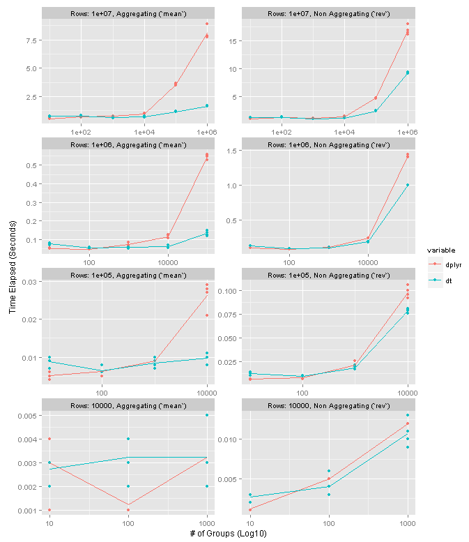
high level results
dplyr and data.table are neck and neck until about 10K groups. Once you get to 100K groups data.table seems to have a 4-5x speed advantage for grouping operations and 1.5x-2x advantage for non-grouping ones. Interestingly it seems that the number of groups is more meaningful in the performance difference as opposed to the size of the groups.
Adding columns seems to have very little effect on the grouping computation, but a substantial impact on the non-grouping one. Here are the results for the 10MM row data frame with one vs. three columns:
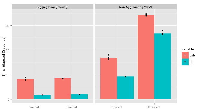
testing more columns
Vs. Base
I also ran some tests for base, focusing only on the 1MM row data frame with 100K groups (note these tests were run on a different machine, though same package versions). Here are the commands I compared:
# Aggregating

aggregate(DF$V.1, DF[1], mean)
data.table(DF)[, mean(V.1), by=G.10]
DF %>% group_by(G.10) %>% summarise(mean(V.1))

# Non-Aggregating

DF$res <- ave(DF$V.1, DF$G.10, FUN=rev)))
data.table(DF)[, res:=rev(V.1), by=G.10]
DF %>% group_by(G.10) %>% mutate(res=rev(V.1))</pre>
And the results: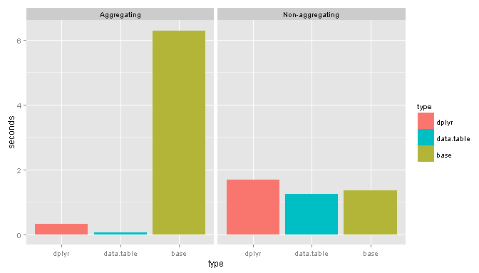
base packages
Suprisingly for non-aggregating tasks base performs remarkably well.
Conclusions
As I’ve noted previously I’m currently a data.table user, and based on these tests I will continue to be a data.table user, particularly because I am already familiar with the syntax. Under some circumstances data.table is definitely faster than dplyr, but those circumstances are narrow enough that they needn’t be the determining factor when chosing a tool to perform split apply combine style analysis.
Both packages work very well and offer substantial advantages over base R functionality. You will be well served with either. If you find one of them is not able to perform the task you are trying to do, it’s probably worth your time to see if the other can do it (please comment here if you do run into that situation).